FDTD electromagnetic field analysis software : Wsf
To Japanese
● 1. Calculation principle and Yee grid
● 2. Types of boundary conditions, PBC and PML
● 3. Types of oscillating direction, one direction and both directions
● 4. Types of oscillating waveforms, pulse and CW
● 5. Calculation for a far field
● 6. Dispersive material calculations
● 7. Measurement of light amount
● 8. Calculation for a scattering field and 360-degree far field
● 9. Calculation of a frequency spectrum
● 10. Cross-sections for various structures
● 11. Calculation for lens focusing
● 12. Visualizing the calculation results
● 13. Output files New 2024/11/12
● Maxwell's equations
● Yee grid and electromagnetic field vector
● difference formulas
● Calculation flow

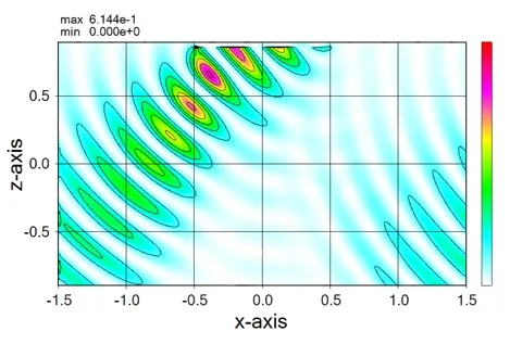
● In the case of a perfectly matched layer (PML).
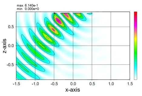
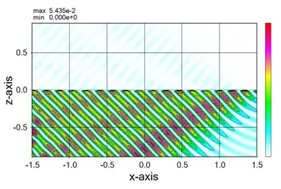
● In the case of bidirectional oscillation.
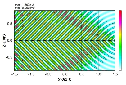
● In the case of laterally unidirectional oscillation.
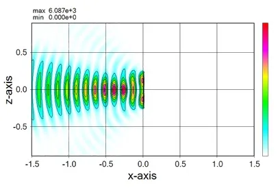

● Example of CW oscillation.

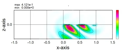
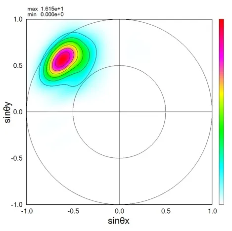
● The far field pattern in the downward direction is calculated for the model shown above.
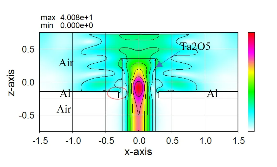
● Wsf has applied the PLRC methodology, including in the PLM domain, to achieve stable calculations even for dispersible materials.
● Measurement result for each material region.

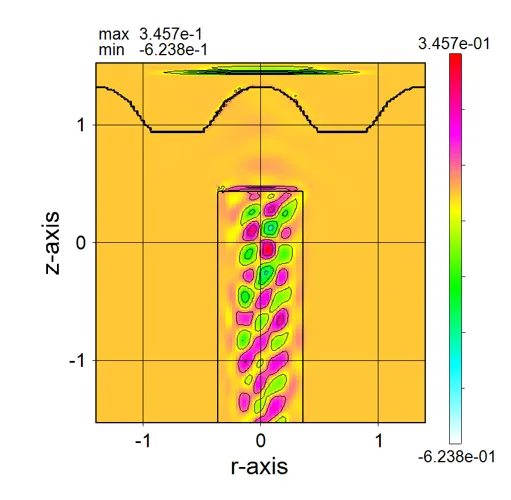
● The 360-degree far field pattern is calculated for the model shown above.
● The wavelength dependence of reflectance and transmittance appear in the frequency spectrum.
● In the case of external definition using sub.dat.
The isolated structure can be defined by the four points (x1,y1), (x2,y2), (x3,y3), and (x4,y4) described in sub.dat.
The structure defined by the piled data of four points. A periodic pattern for these structures can be defined easily.
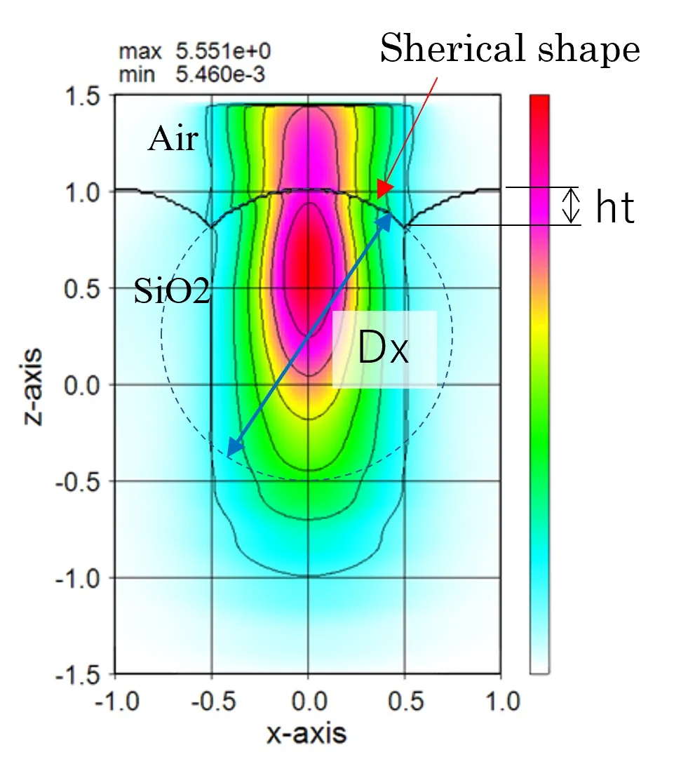
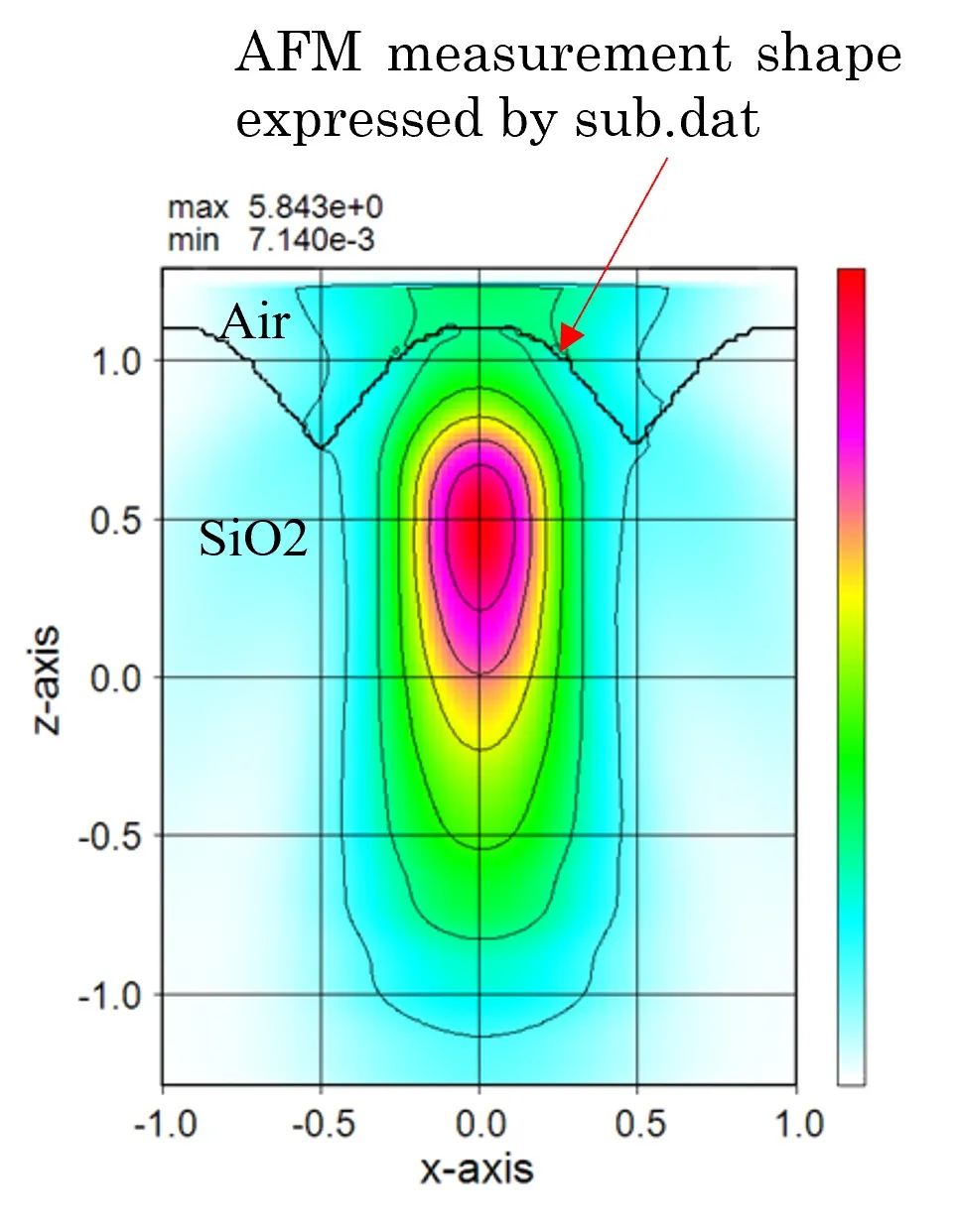
● The lens shape is expressed by stacking the externally defined circular structure.
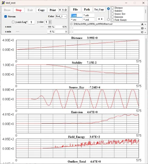
● Displayed by Wsmnt.
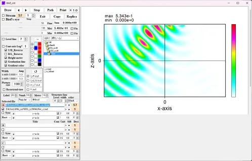
● Displayed by Wscnt.
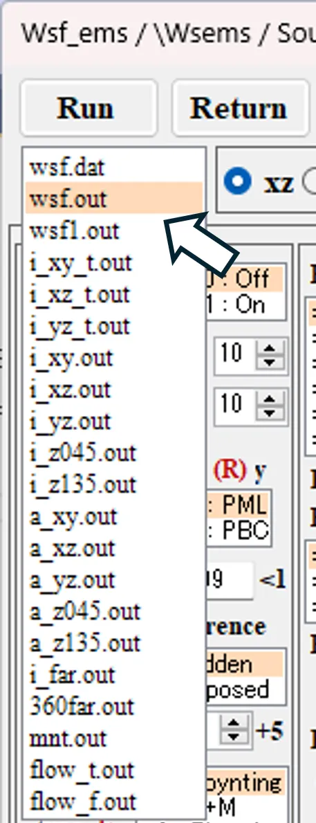
● wsf.out Main calculation results.
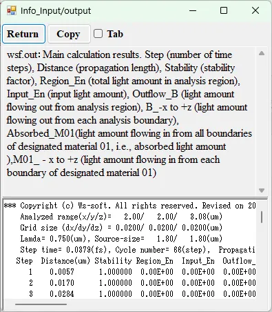
● wsf1.out Extracted calculation results.
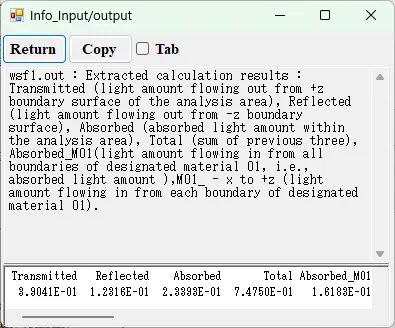
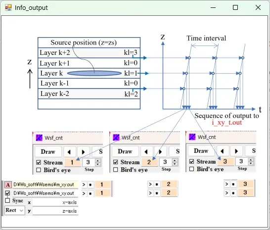
● i_xy_t.out xy cross-sectional distributions of light intensity (i. e., magnitude of Poynting vector) at fixed intervals.
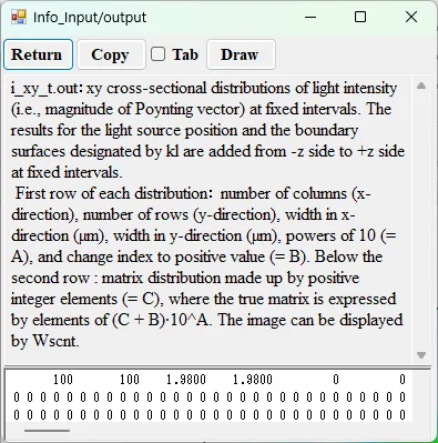
drawing example.
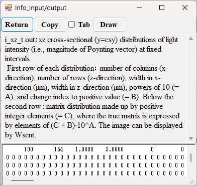
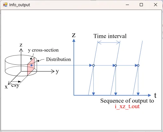
● i_xz_t.out xz cross-sectional (y=csy) distributions of light intensity at fixed intervals.
drawing example.
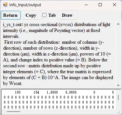
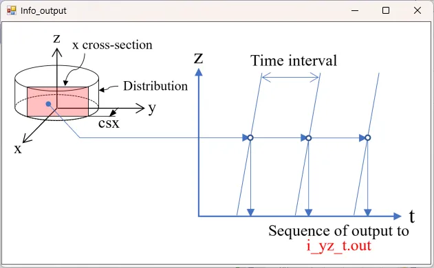
● i_yz_t.out yz cross-sectional (x=csx) distributions of light intensity at fixed intervals.
drawing example.
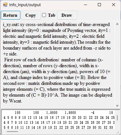
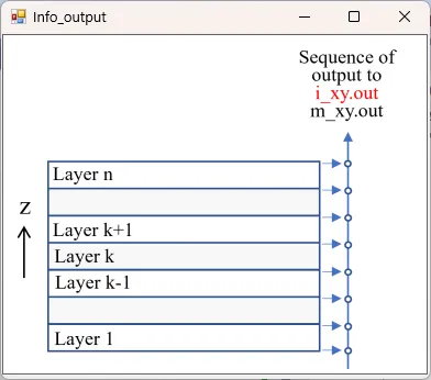
● i_xy.out xy cross-sectional time-averaged distributions of light intensity.
drawing example.
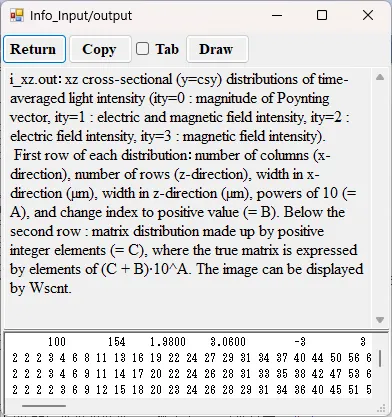
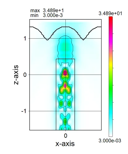
● i_xz.out xz cross-sectional (y=csy) time-averaged distributions of light intensity.
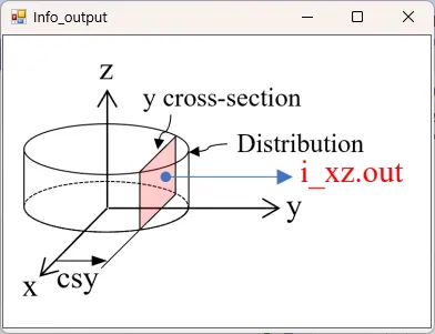
drawing example.
● i_yz.out yz cross-sectional (x=csx) time-averaged distributions of light intensity.
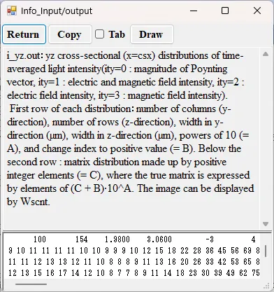
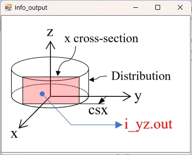
drawing example.
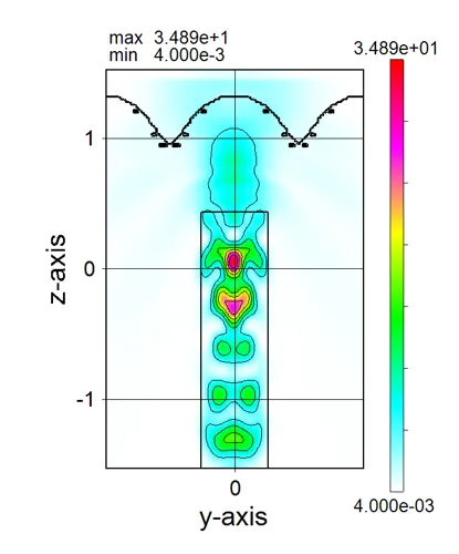
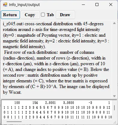
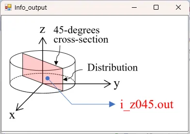
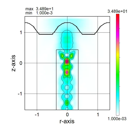
● i_z045.out Cross-sectional distribution with 45-degrees rotation around z-axis for light intensity.
drawing example.
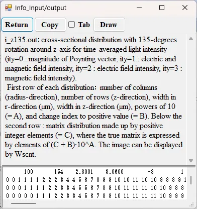
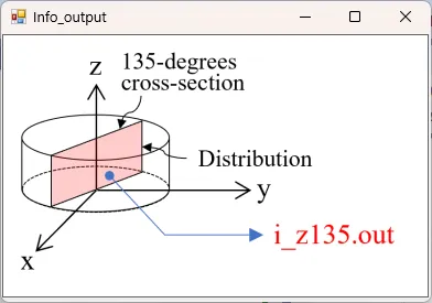
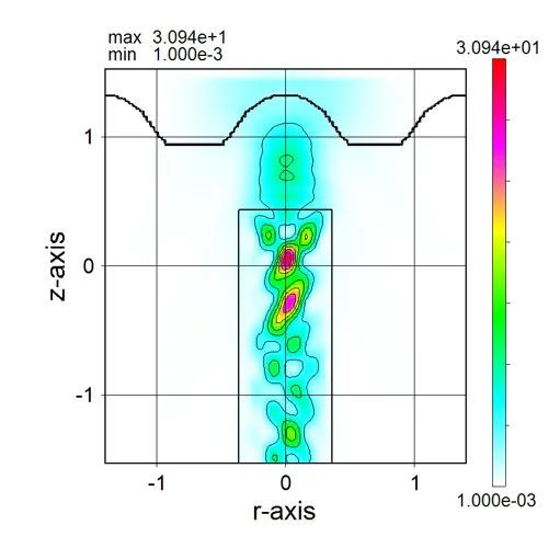
● i_z135.out Cross-sectional distribution with 135-degrees rotation around z-axis for light intensity.
drawing example.
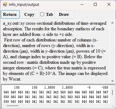
● a_xy.out xy cross-sectional time-averaged distributions of absorption.
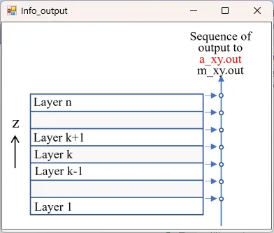
drawing example.
● a_xz.out xz cross-sectional (y=csy) time-averaged distributions of absorption.
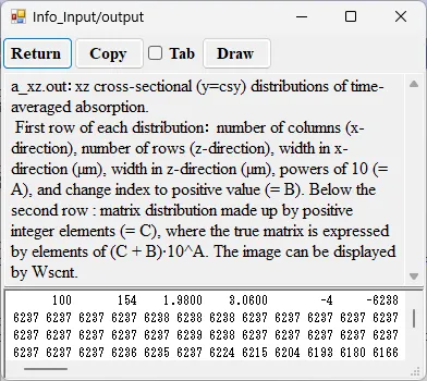
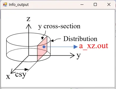
drawing example.
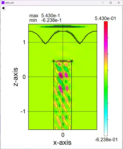
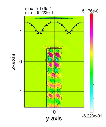
● a_yz.out yz cross-sectional (x=csx) time-averaged distributions of absorption.
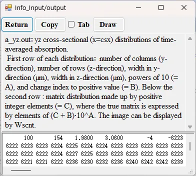
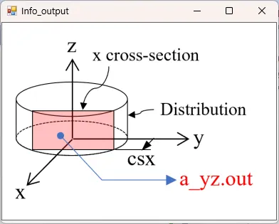
drawing example.
● a_z045.out Cross-sectional distribution with 45-degrees rotation around z-axis for absorption.
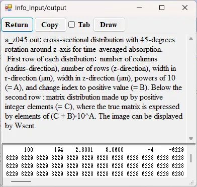
drawing example.
● a_z135.out Cross-sectional distribution with 135-degrees rotation around z-axis for absorption.
drawing example.
● i_far.out Far-field intensity distributions (-z side and +z side in the order).
drawing example.
● 360far.out 360-degree far-field distributions.
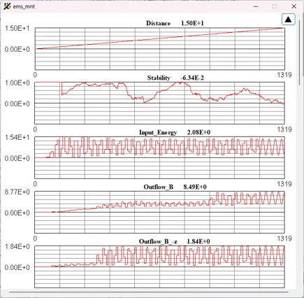
● mnt.out Output for Wsmnt.
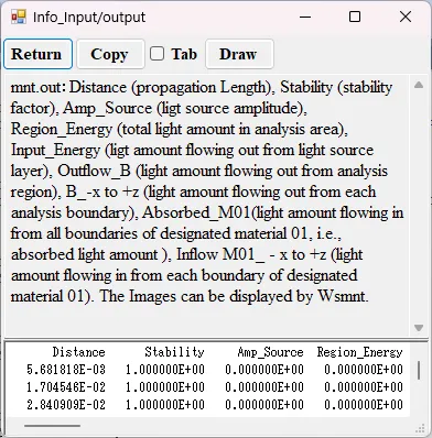
drawing example.
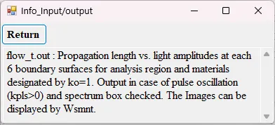
● flow_t.out Light amplitudes for propagation length at each 6 boundary surfaces.
● flow_f.out Fourier-transform of light amplitudes.

● 2. Types of boundary conditions, PBC and PML
● 3. Types of oscillating direction, one direction and both directions
● 4. Types of oscillating waveforms, pulse and CW
● 5. Calculation for a far field
● 6. Dispersive material calculations
● 7. Measurement of light amount
● 8. Calculation for a scattering field and 360-degree far field
● 9. Calculation of a frequency spectrum
● 10. Cross-sections for various structures
● 11. Calculation for lens focusing
● 12. Visualizing the calculation results
● 13. Output files New 2024/11/12
1. Calculation principle and Yee grid ▲top
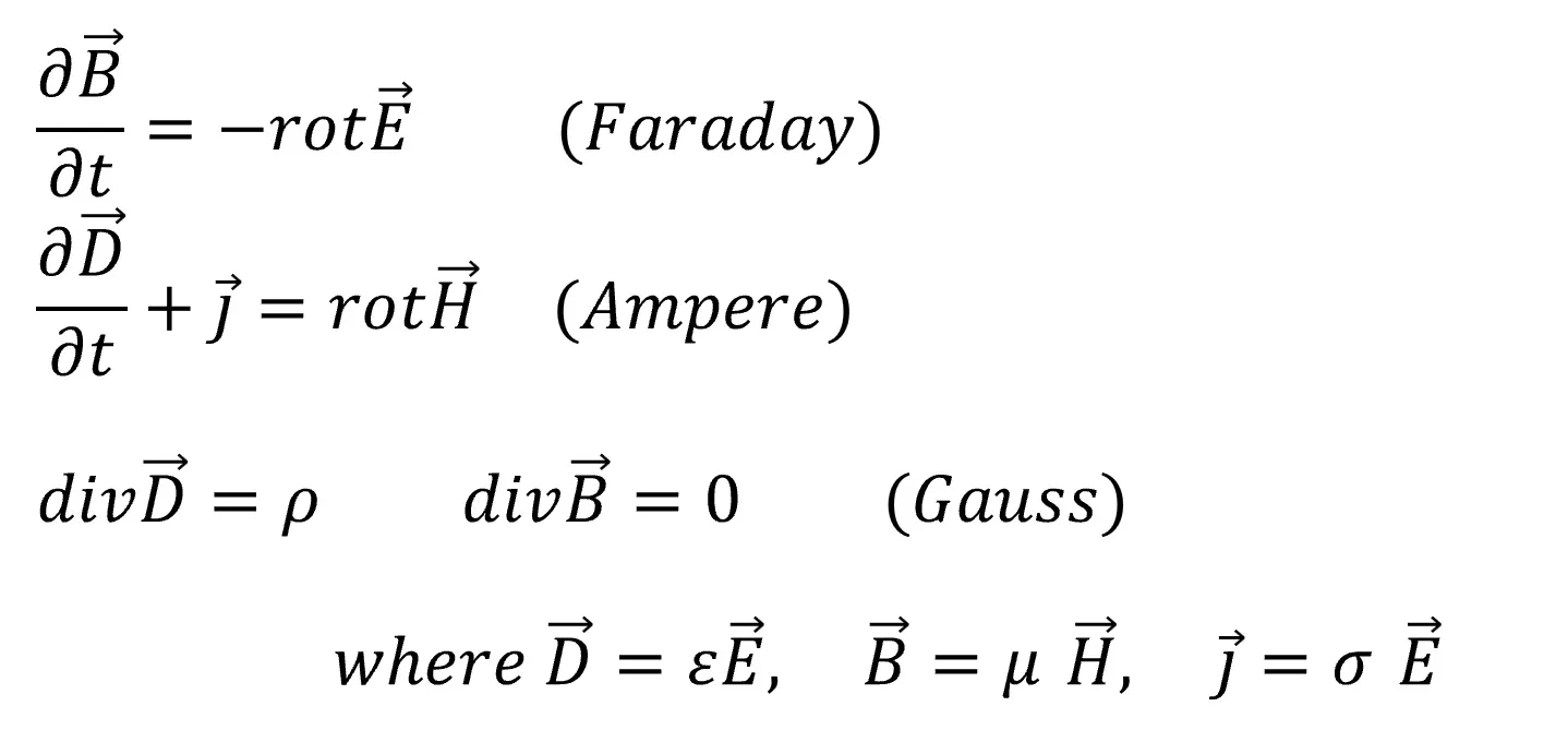
Wsf uses the calculation principle of FDTD (Finite Difference Time Domain), which sequentially solves the difference equations of Maxwell's equations in the time domain based on the arrangement of electromagnetic field vectors in the Yee grid.● Maxwell's equations

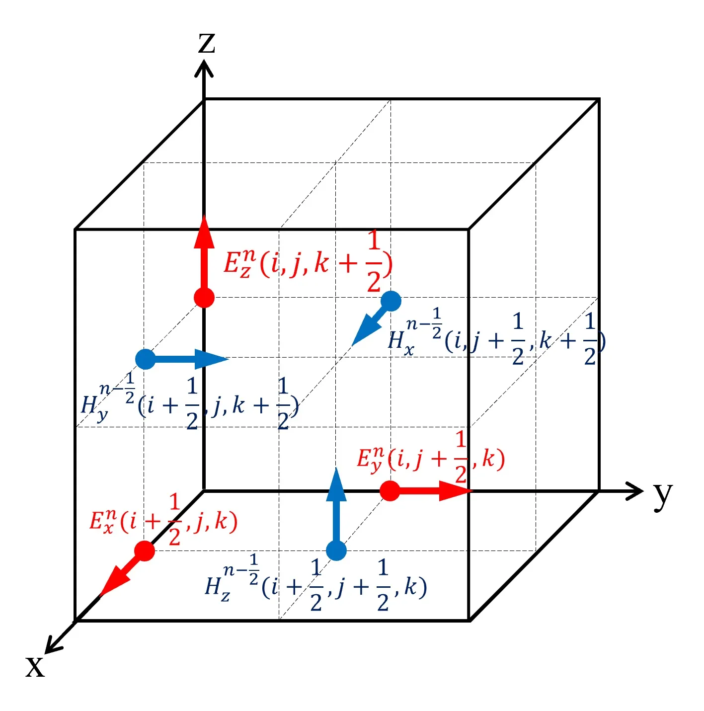
● Yee grid and electromagnetic field vector

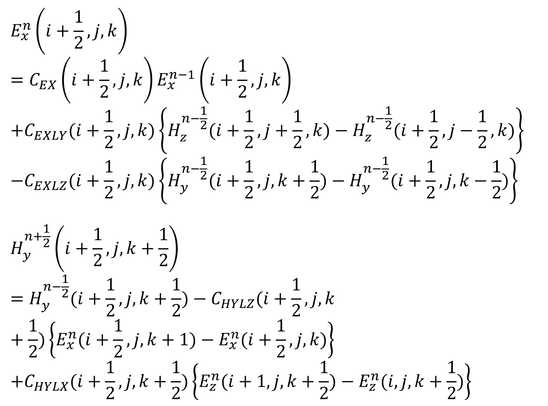
● difference formulas

● Calculation flow

2. Types of boundary conditions, PBC and PML ▲top
● In the case of a periodic boundary condition (PBC).
● In the case of a perfectly matched layer (PML).

3. Types of oscillating direction, one direction and both directions ▲top
● In the case of unidirectional oscillation.
● In the case of bidirectional oscillation.

● In the case of laterally unidirectional oscillation.

4. Types of oscillating waveforms, pulse and CW ▲top
● Example of pulse oscillation.
● Example of CW oscillation.

5. Calculation for a far field ▲top
● Inclined CW light is oscillated from the middle surface to the bottom surface.
● The far field pattern in the downward direction is calculated for the model shown above.

6. Dispersive material calculations ▲top
In many dispersive materials such as Al, the decay coefficient is larger than the refractive index, and the FDTD algorithm runs out of control.● Wsf has applied the PLRC methodology, including in the PLM domain, to achieve stable calculations even for dispersible materials.

7. Measurement of light amount ▲top
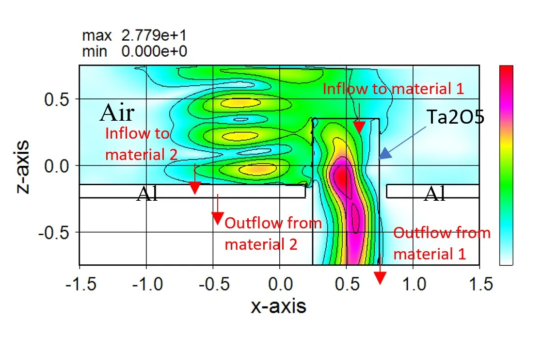
● The amount of light input and output and the amount of light absorbed can be measured individually for each material or area.
● Measurement result for each material region.
8. Calculation for a scattering field and 360-degree far field ▲top
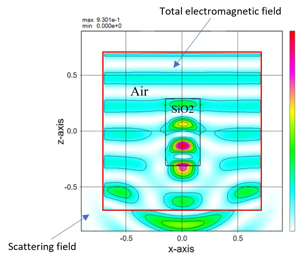
● The scattered field can be calculated separately from the total electromagnetic field.
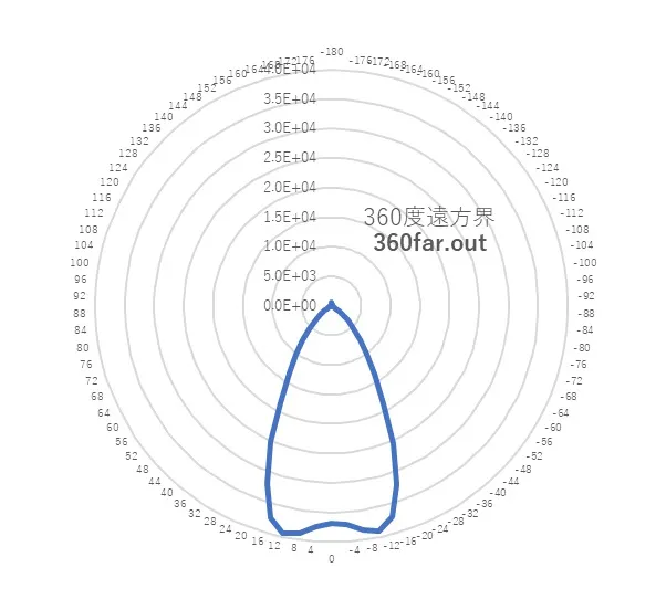
● The 360-degree far field pattern is calculated for the model shown above.

9. Calculation of a frequency spectrum ▲top
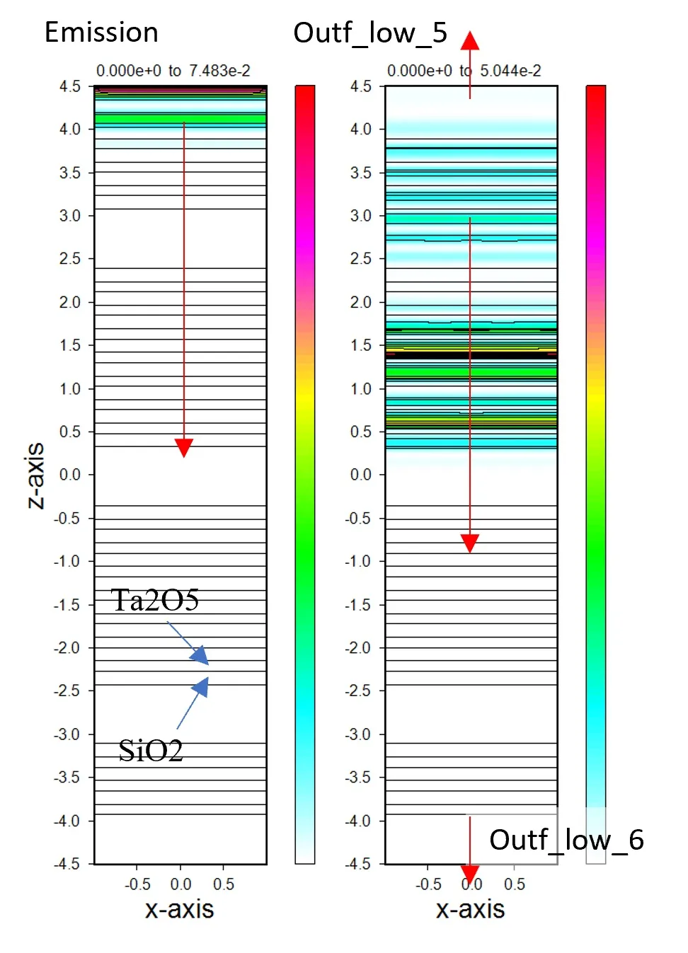
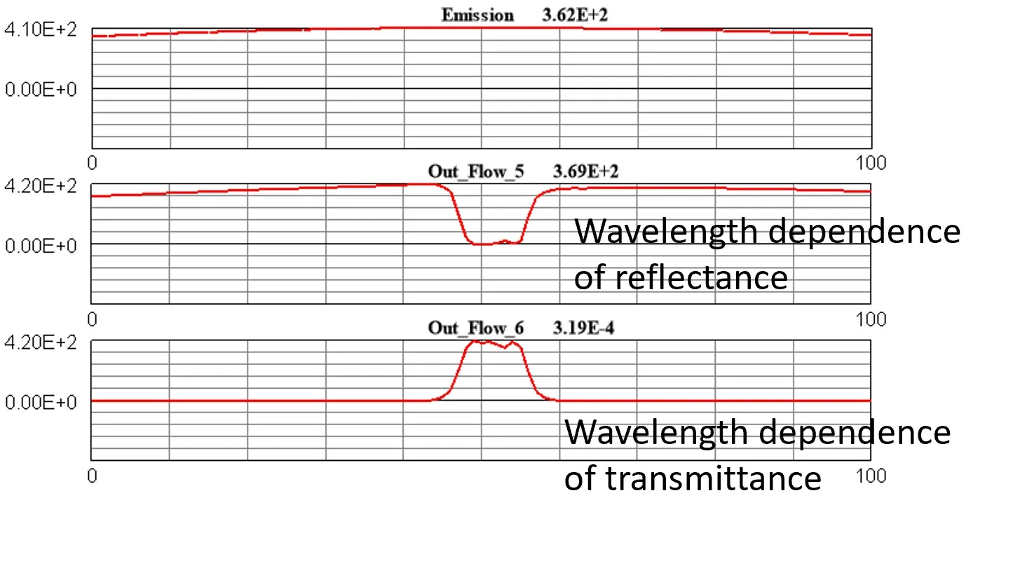
● Example of frequency response calculation for BPF using pulse oscillation.
● The wavelength dependence of reflectance and transmittance appear in the frequency spectrum.

10. Cross-sections for various structures ▲top
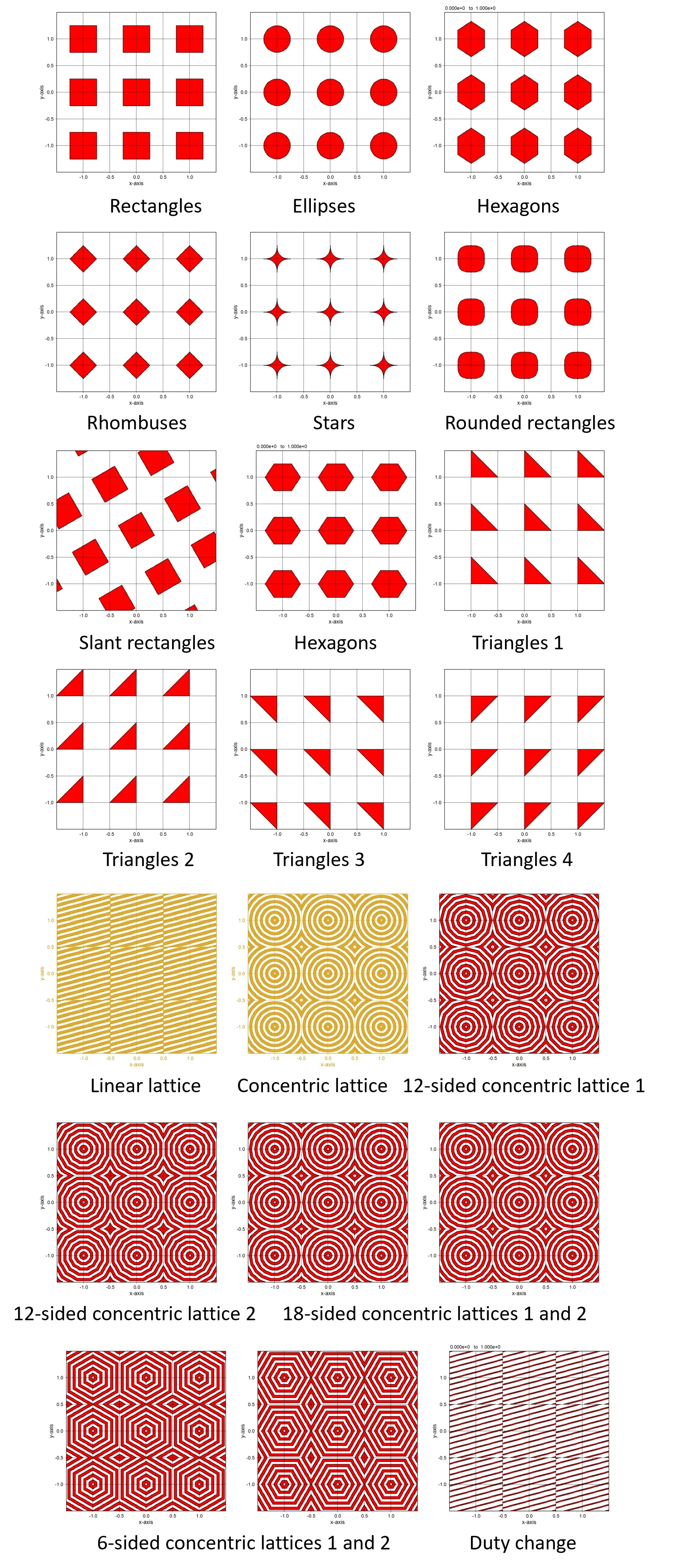
● In the case of internal definition.
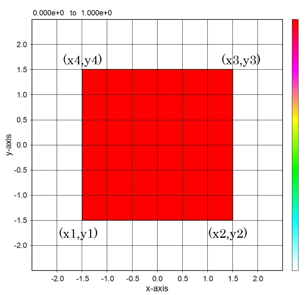
● In the case of external definition using sub.dat.
The isolated structure can be defined by the four points (x1,y1), (x2,y2), (x3,y3), and (x4,y4) described in sub.dat.

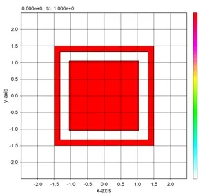
The structure defined by the piled data of four points. A periodic pattern for these structures can be defined easily.

11. Calculation for lens focusing ▲top
● The lens shape is expressed by stacking the internally defined circular structure.
● The lens shape is expressed by stacking the externally defined circular structure.

12. Visualizing the calculation results ▲top
At runtime, the calculation results are displayed in real time by Wsmnt and Wscnt.● Displayed by Wsmnt.

● Displayed by Wscnt.

13. Output files ▲top
The contents of each output file are described based on the contents displayed by double-clicking the item in the Result file box on the Source setting window.
● wsf.out Main calculation results.

● wsf1.out Extracted calculation results.

● i_xy_t.out xy cross-sectional distributions of light intensity (i. e., magnitude of Poynting vector) at fixed intervals.


drawing example.
● i_xz_t.out xz cross-sectional (y=csy) distributions of light intensity at fixed intervals.


drawing example.
● i_yz_t.out yz cross-sectional (x=csx) distributions of light intensity at fixed intervals.


drawing example.
● i_xy.out xy cross-sectional time-averaged distributions of light intensity.


drawing example.
● i_xz.out xz cross-sectional (y=csy) time-averaged distributions of light intensity.


drawing example.

● i_yz.out yz cross-sectional (x=csx) time-averaged distributions of light intensity.


drawing example.

● i_z045.out Cross-sectional distribution with 45-degrees rotation around z-axis for light intensity.


drawing example.

● i_z135.out Cross-sectional distribution with 135-degrees rotation around z-axis for light intensity.


drawing example.

● a_xy.out xy cross-sectional time-averaged distributions of absorption.


drawing example.
● a_xz.out xz cross-sectional (y=csy) time-averaged distributions of absorption.


drawing example.

● a_yz.out yz cross-sectional (x=csx) time-averaged distributions of absorption.


drawing example.

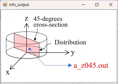
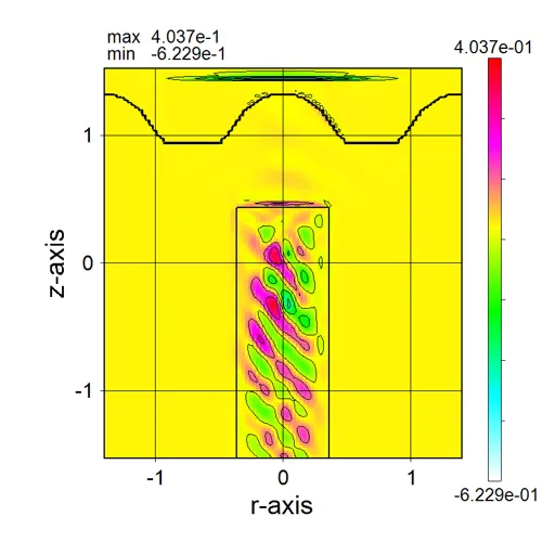
● a_z045.out Cross-sectional distribution with 45-degrees rotation around z-axis for absorption.


drawing example.

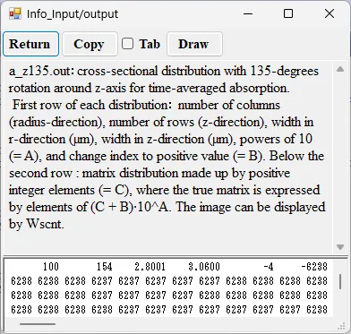
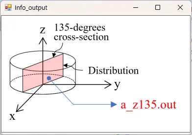
● a_z135.out Cross-sectional distribution with 135-degrees rotation around z-axis for absorption.


drawing example.

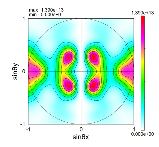
● i_far.out Far-field intensity distributions (-z side and +z side in the order).

drawing example.

● 360far.out 360-degree far-field distributions.

● mnt.out Output for Wsmnt.

drawing example.

● flow_t.out Light amplitudes for propagation length at each 6 boundary surfaces.

● flow_f.out Fourier-transform of light amplitudes.
