Installation and basic usage of Ws_soft
To Japanese
● 1. How to install Ws_soft New 2025/11/27
● 2. Usage examples using sample data
● 3. Sample calculation examples
● 4. Viewing information about parameters and buttons
● 5. Basic operation of the structure settings panel
● 6. Structure definition
● 7. Output files in the definition structure
● 8. Wave calculation
● 9. Limitation
Learn more
● 10. Material Data Settings (nk.dat)
● 11. Structural Auxiliary Data Settings (sub.dat)
● 12. Serial Caluculation (Wsbch)
● 13. Identification and correction of incorrect input
● 14. Light amount detection
(2) Remove the folder of Ws_soft from the drive to uninstall the software.
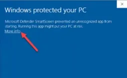
(2) If the protection window appears, click on 'More info', and then click the run button that appears in the lower left corner.
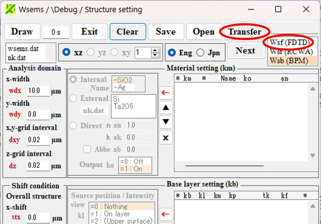
(3) After the Structure setting window of Wsems appears, select Wsf (FDTD) in it and click the Transfer button.
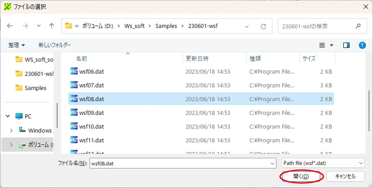
(4) On the file selection window, select a file (wsf08.dat) from the '\Samples\230601-wsf' directory and click the Open button.
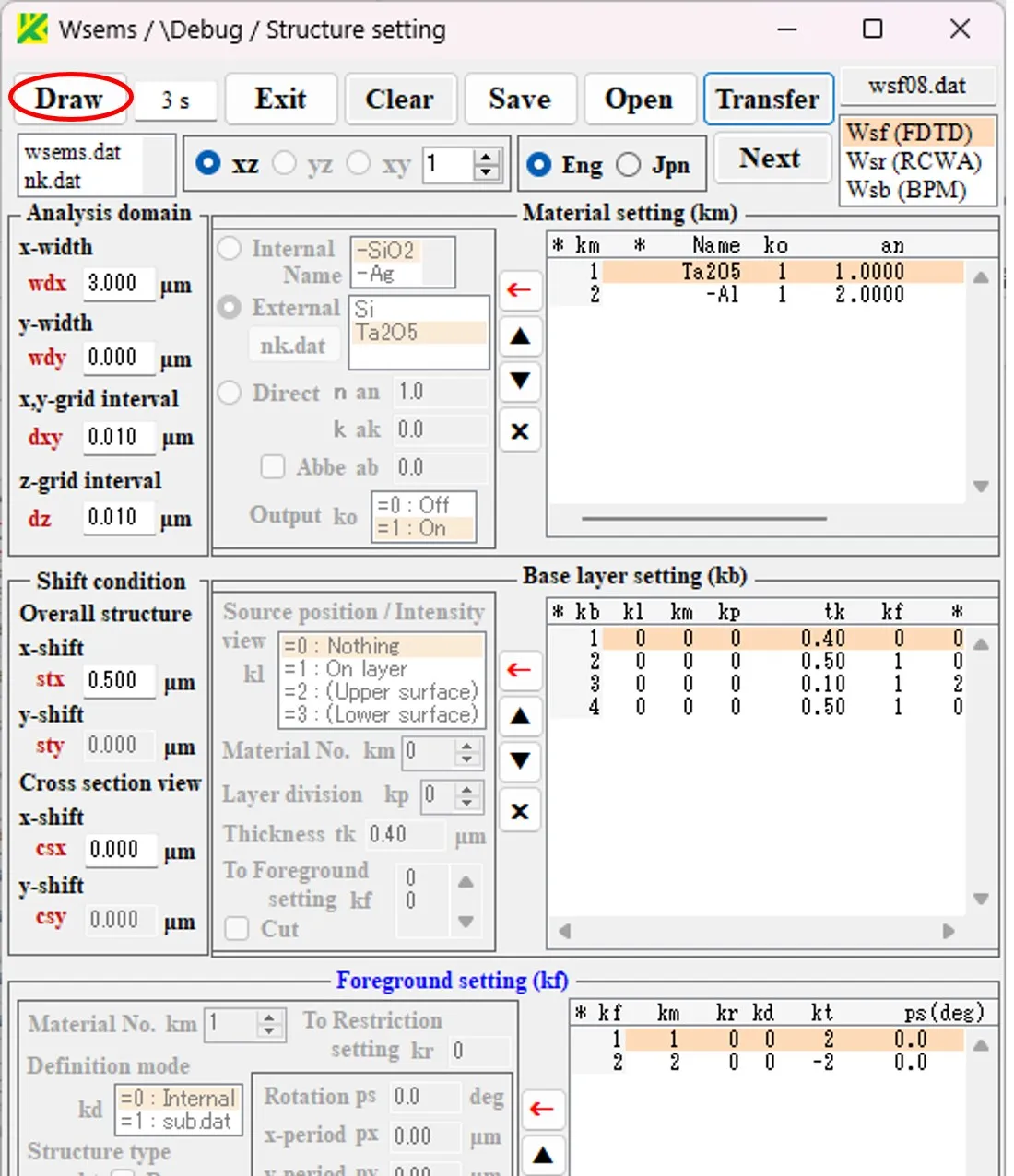
(5) The Structure setting window is updated and click the Draw button.
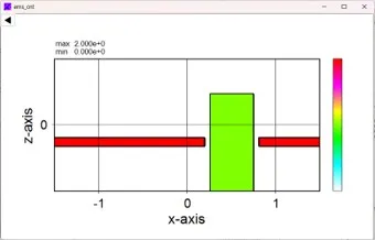
(6) The Wscnt window appears and the cross-sectional shape is displayed.
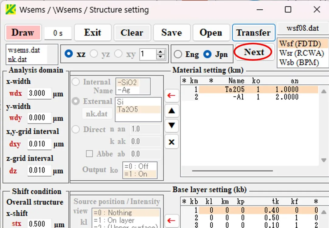
(7) On the Structure setting window, click the Next button.
(8) The Source setting window appears, and click the Transfer button in it.
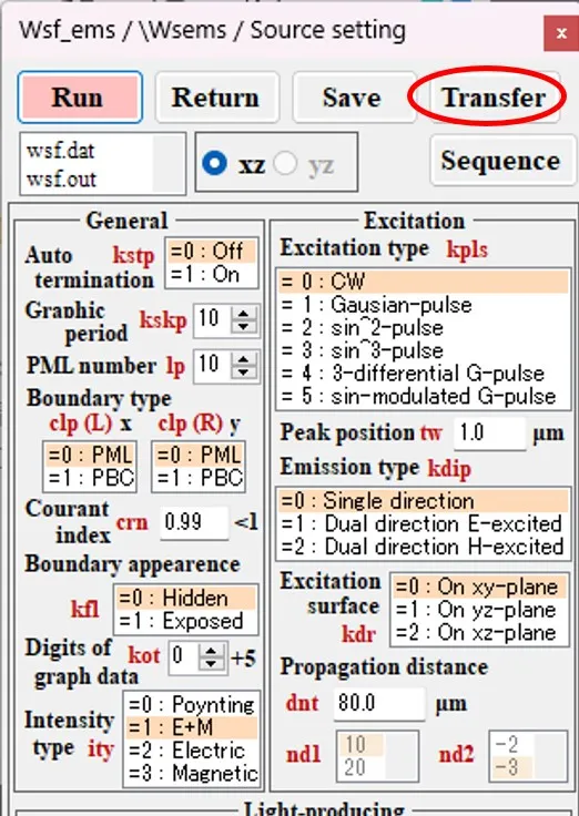
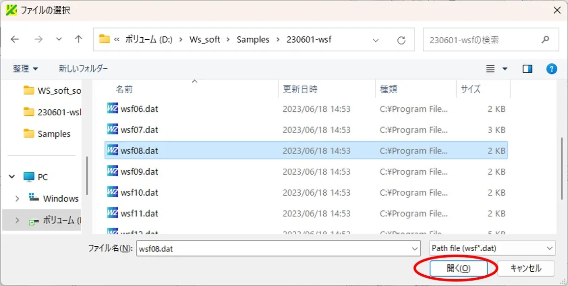
(9) On the file selection window, select a file (wsf08.dat) from the '\Samples\230601-wsf' directory and click the Open button.
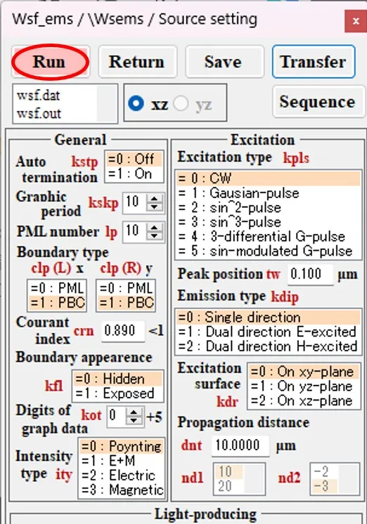
(10) The Source setting window is updated and click the Run button.
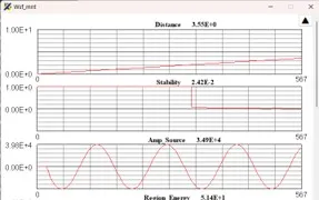
(11) The Wsmnt window and the Wscnt window appear, and the calculation progress and cross-sectional intensity distribution are displayed in real time.
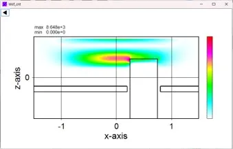
(12) Move the mouse pointer over the result file box on the Source setting window.
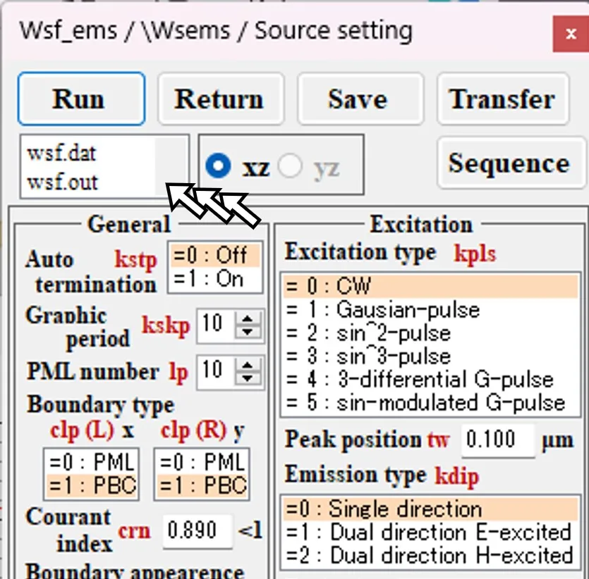
(13) The result file box expands downward.
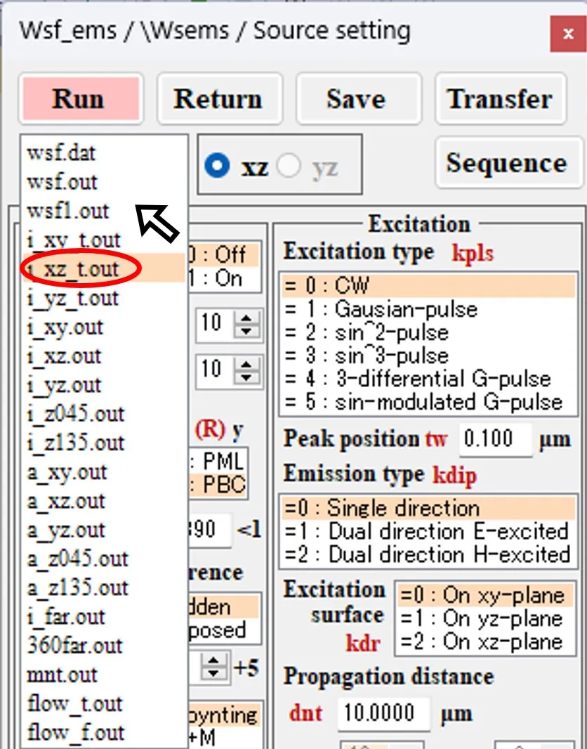
(14) Double-click on one of the files (i_xz_t.out) in the result file box to bring up an information window.
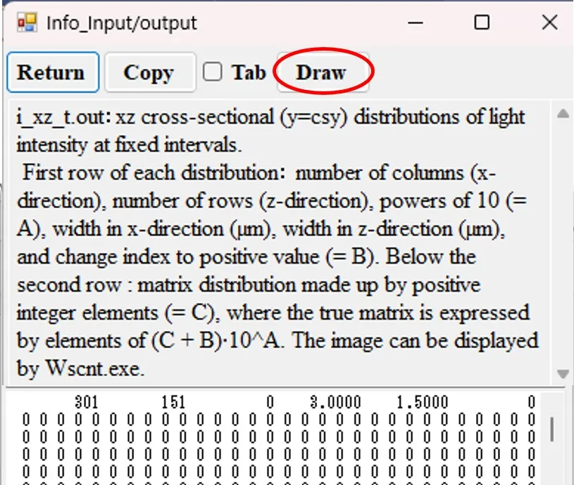
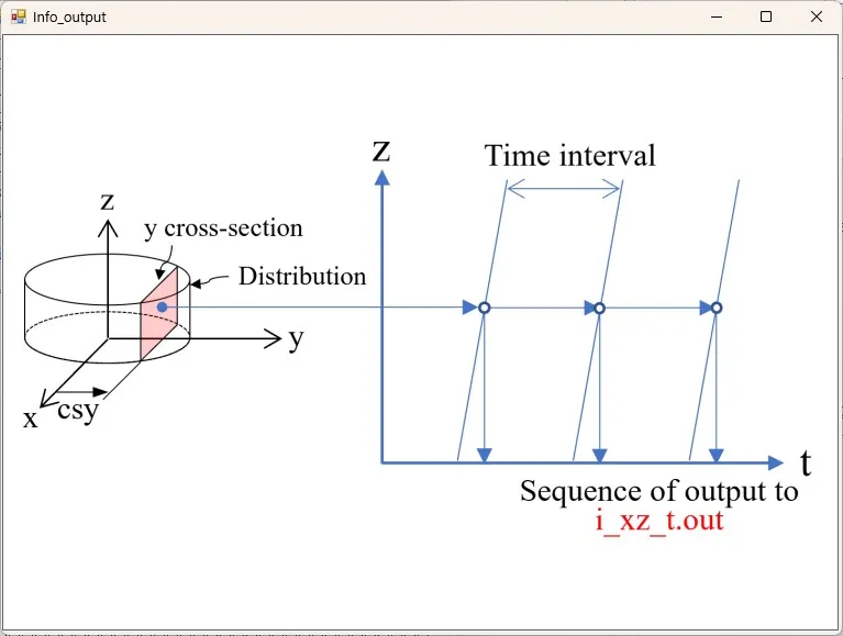
(15) When you click the Draw button, Wscnt is automatically launched and the calculation result is redrawn.
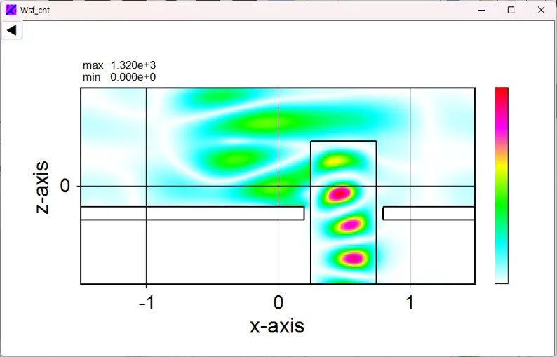
(16) Go back to (12) and double-click one of the files (mnt.out) in the result file box to display the information window.
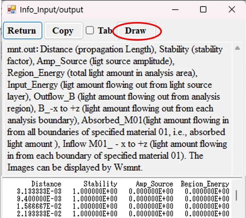
(17) When you click the Draw button, Wsmnt is automatically launched and the calculation result is redrawn.
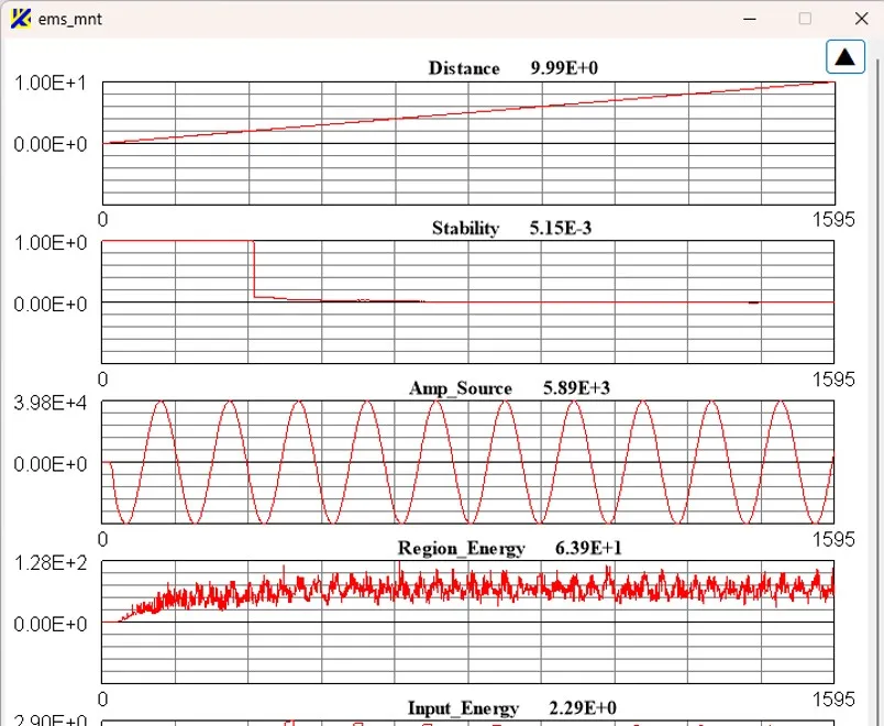
● Calculation examples for sample data in folders of \Samples are shown below.
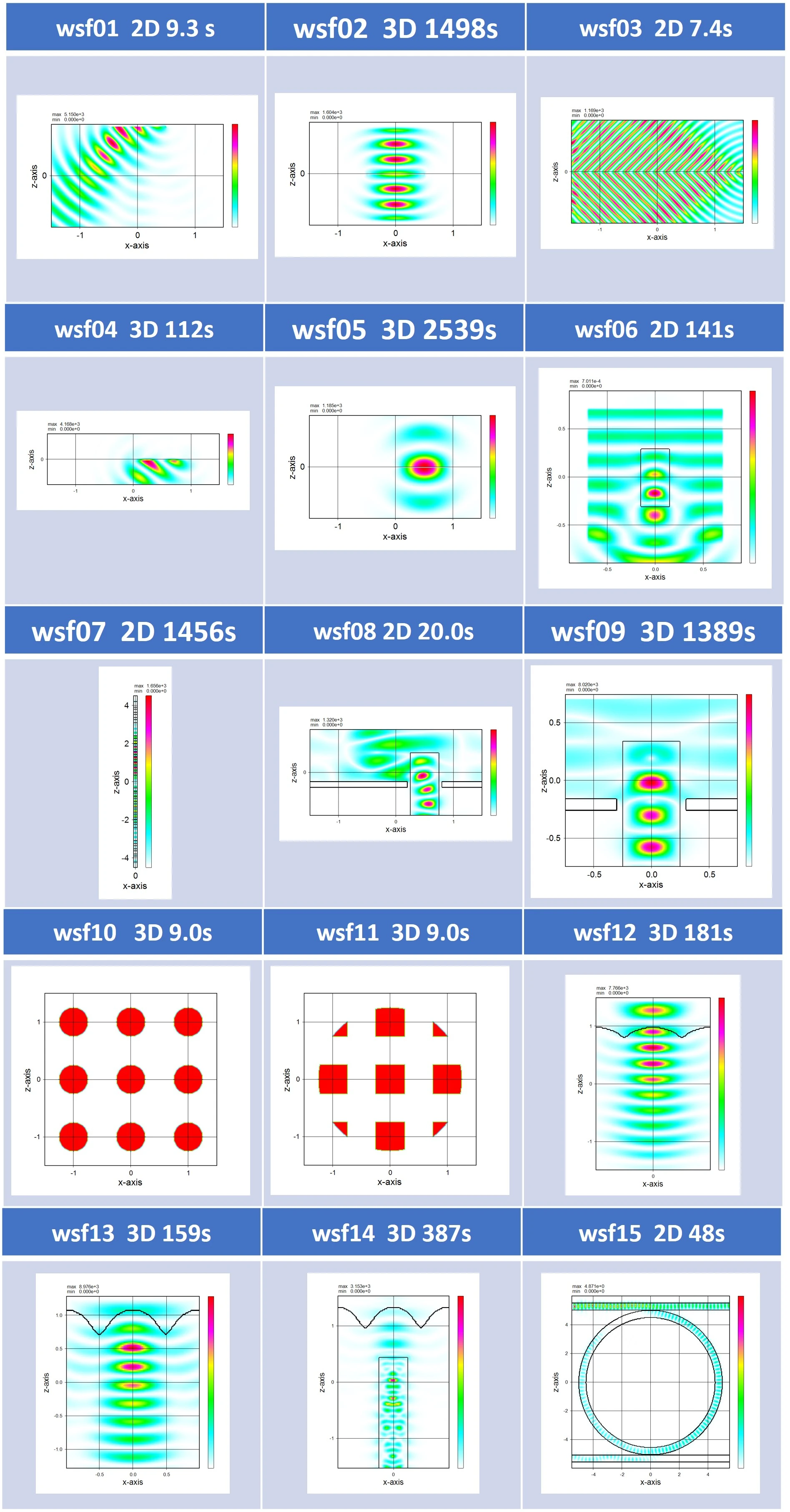
(1) Calculation examples for sample data in \Samples\230601-wsf
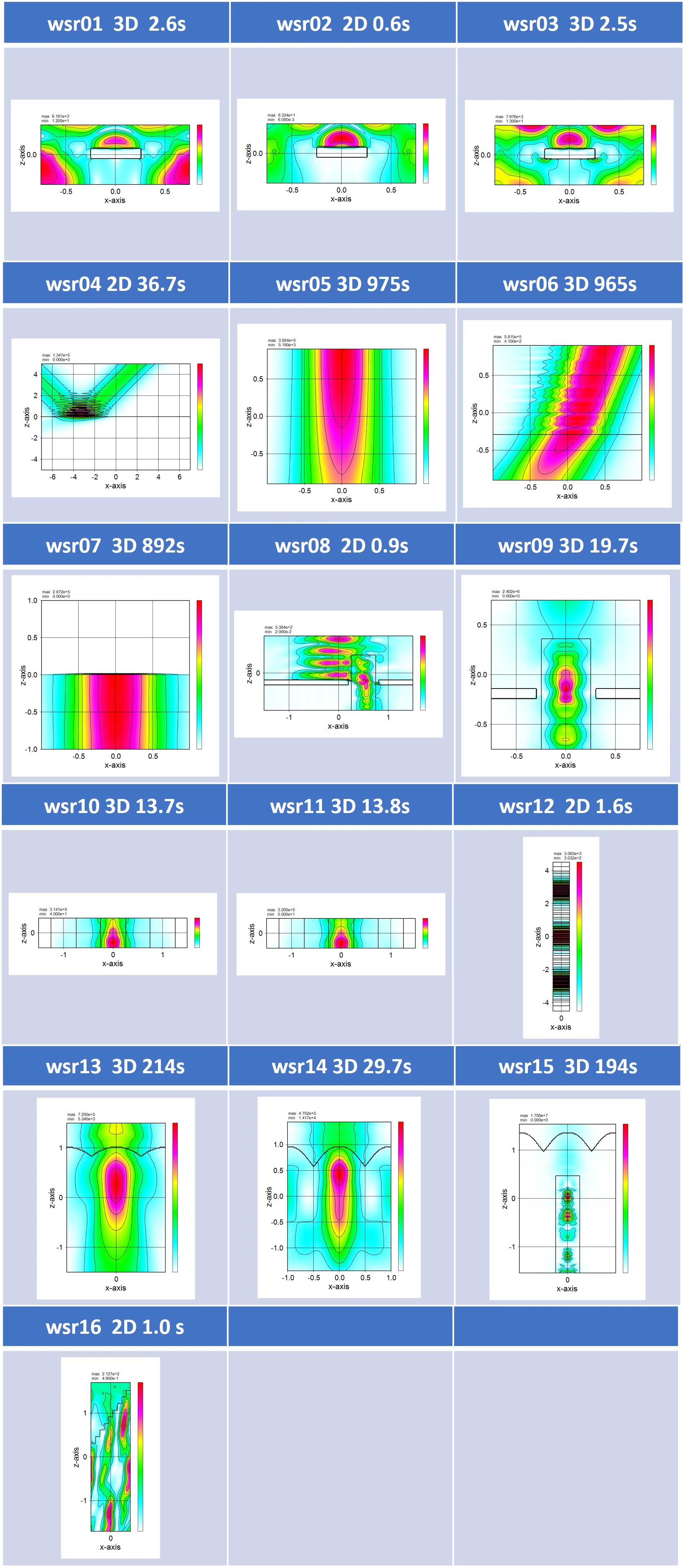
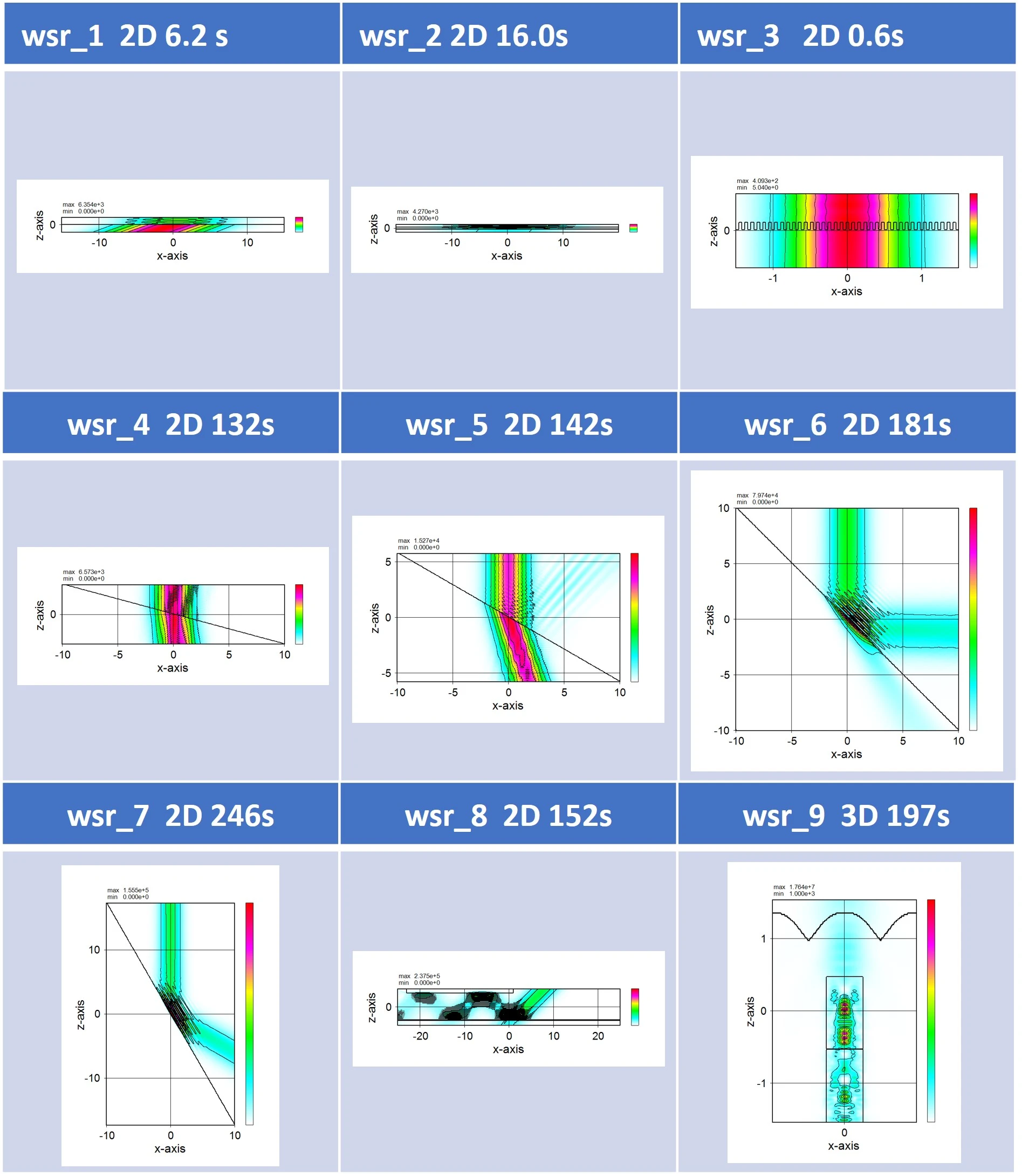
(2) Calculation examples for sample data in \Samples\230601-wsr
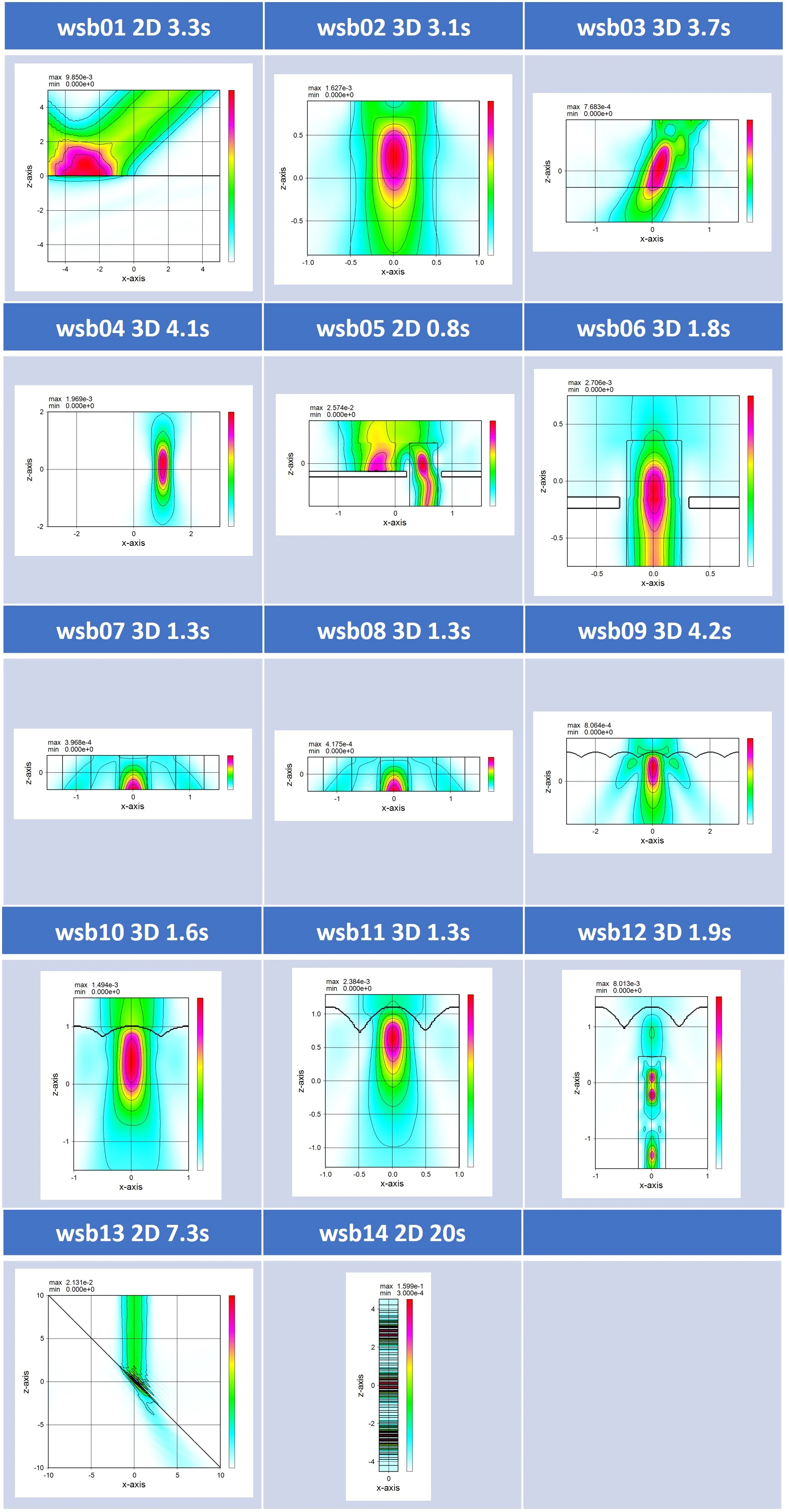
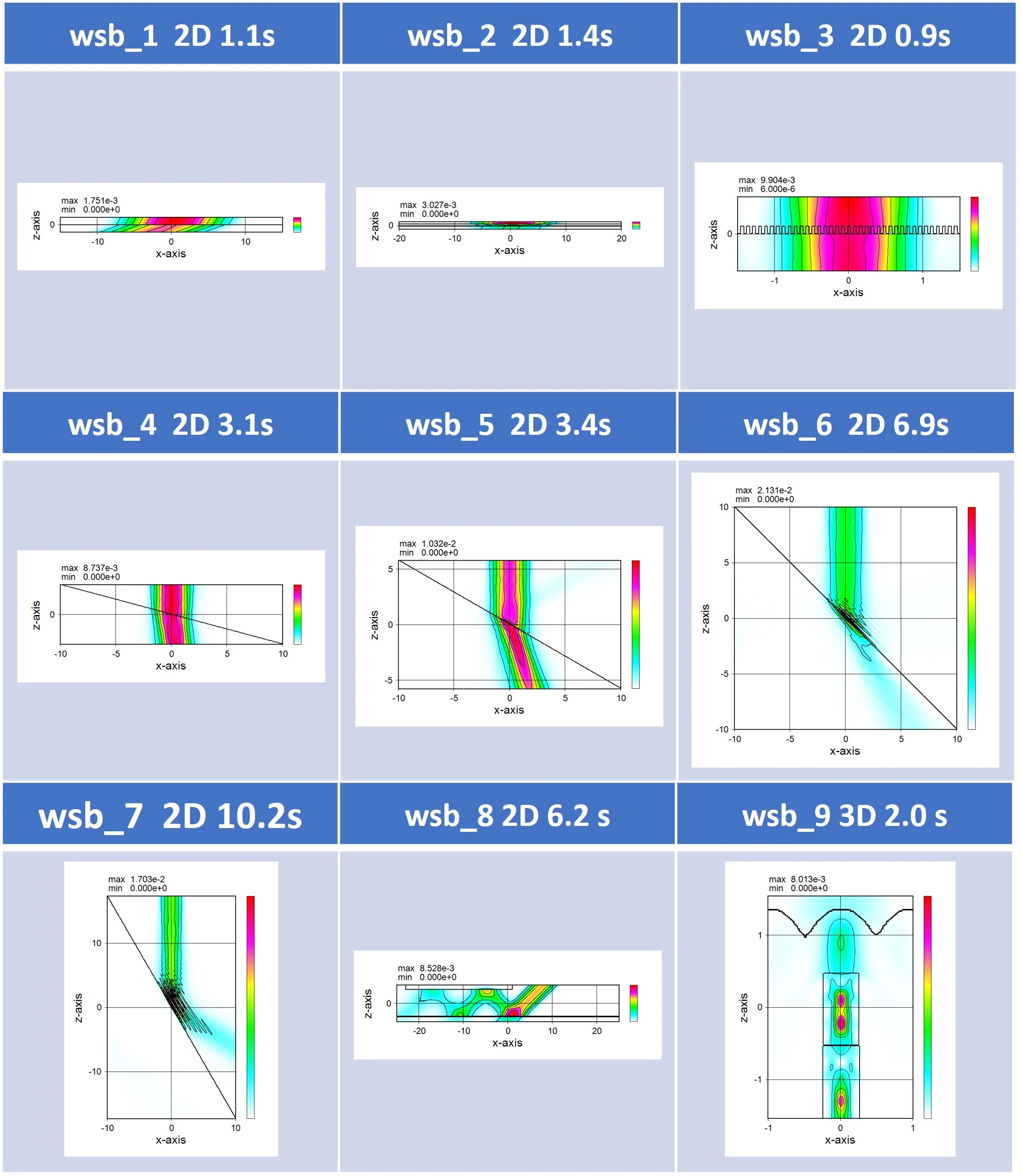
(3) Calculation examples for sample data in \Samples\230601-wsb
● Calculation examples for sample data in folders of \Samples\Comparison are shown below.
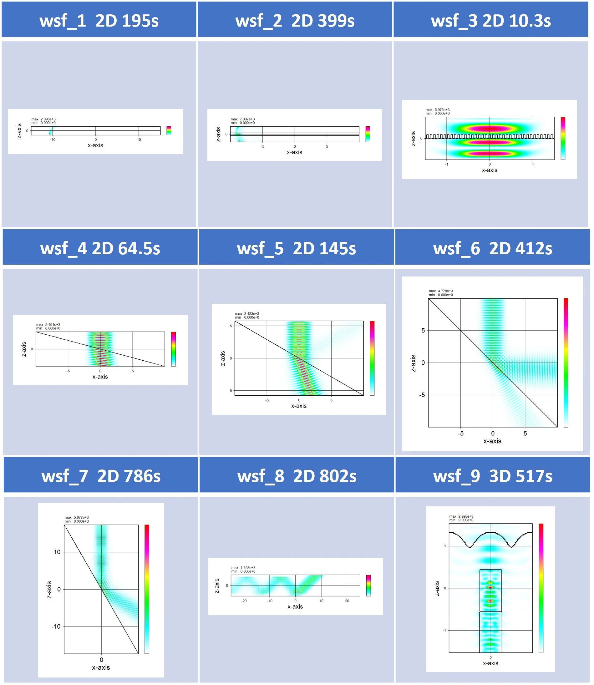
(4) Calculation examples for sample data in \Samples\Comparison\230601-wsf. Paid for only wsf_9.dat (Limitation).
(5) Calculation examples for sample data in \Samples\Comparison\230601-wsr. Paid for only wsr_9.dat (Limitation).
(6) Calculation examples for sample data in \Samples\Comparison\230601-wsb. Paid for only wsb_9.dat (Limitation).
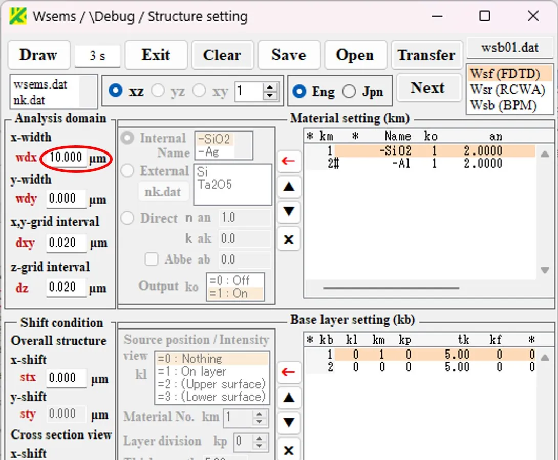
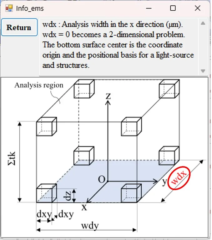
(2) The parameter definition information window (Info) appears, and the corresponding parameter is displayed in red. All parameters in the boxes in the Enable state are double-clicked to display the definition information on the Information window.
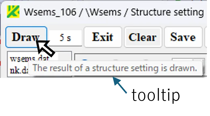
(3) When you hover the mouse pointer over a button in the Enable state, the operating information is displayed in the tooltip.
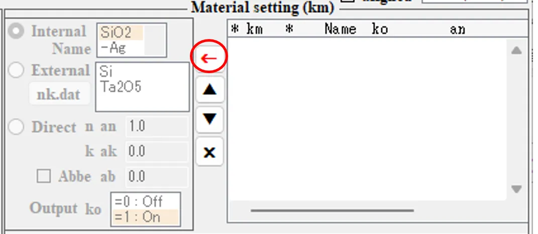
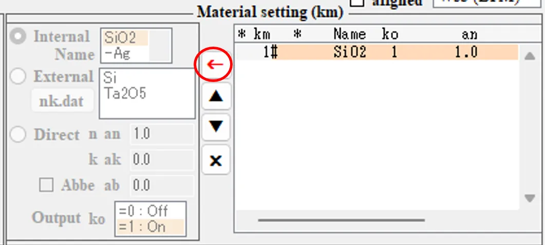
When you click the ← button, the contents of the registration list are moved to the edit panel, and you can edit them.

Clicking on one of the four red buttons completes the edit, and the result of the edit is reflected in the registration list.

Let's take the definition of the material as an example and explain it concretely.
(1) After clicking the Clear button to initialize the panel, click the ← button in the Material setting field.
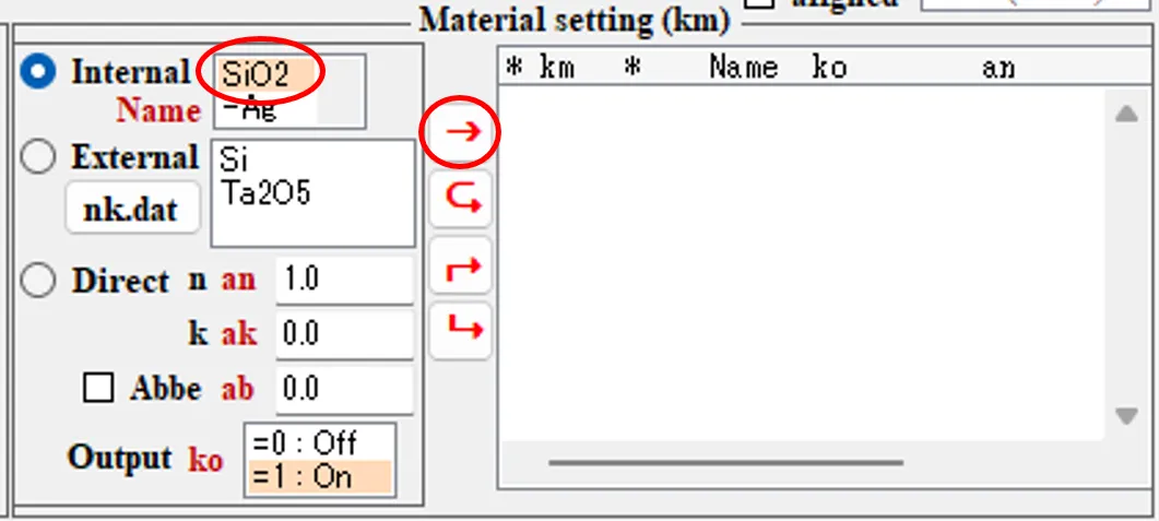
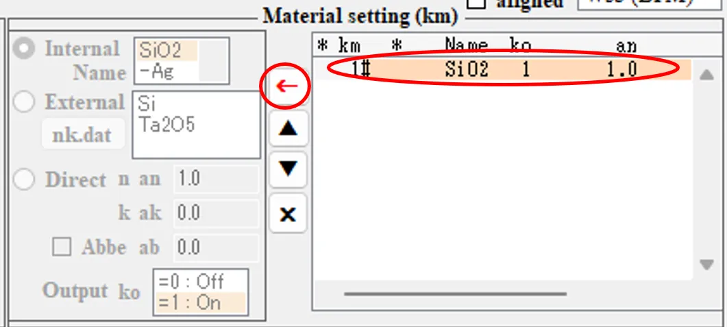
(2) Select SiO2 in the Internal box. Click the → button to register the first line.
(3) Click the ← button in the Base setting field.
(4) Select -Al in the Internal box. Click the ↳ button to register the second line.
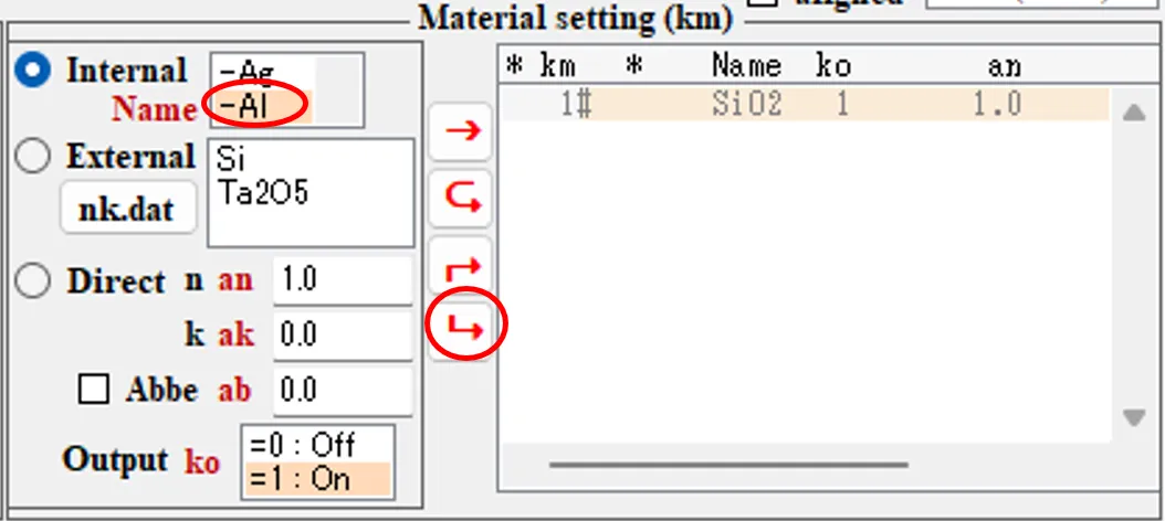
(5) Move the specified item in the registration list up with the ▲ button.
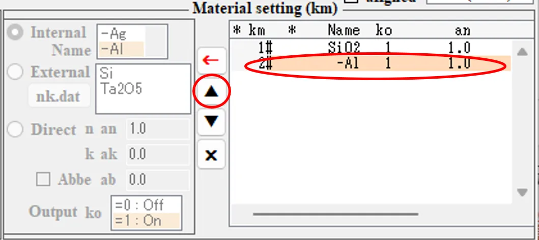
(6) Move the specified item in the registration list down with the ▼ button.
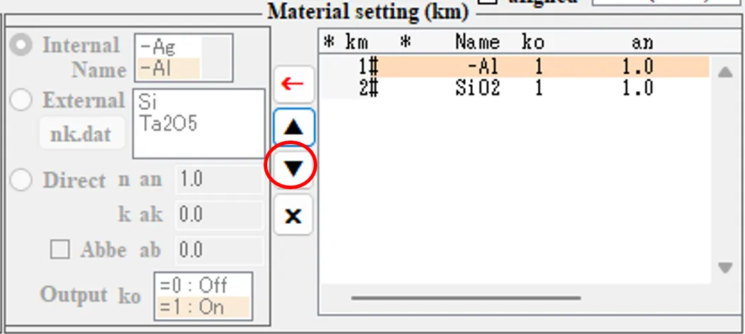
(7) Delete the specified item in the registration list with the × button.
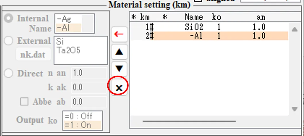
(8) When you click the ← button, the focus shifts to the left and you can edit it.
(9) When you perform an edit operation (-Al selection) on the left side, the → button appears.
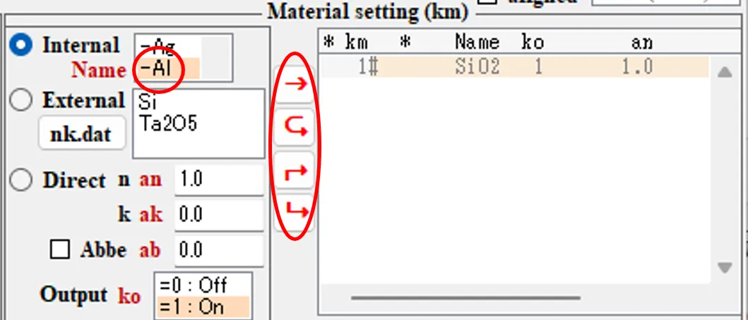
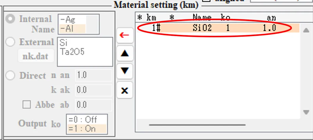
(10) If you click the ⮎ button in (9), the focus will return to the right without reflecting the editing result.
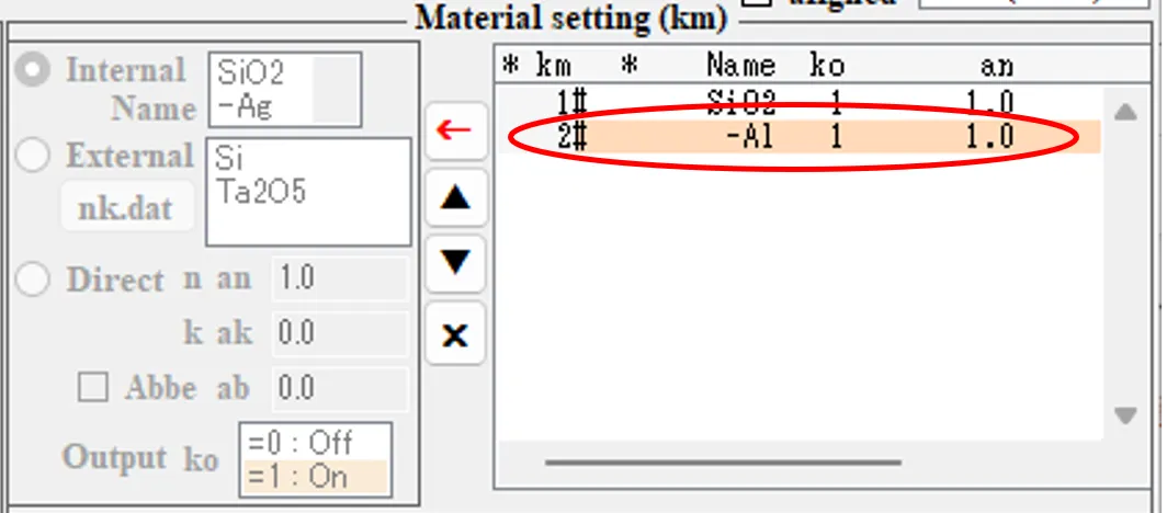
(11) If you click the ↱ button in (9), the editing result will be inserted above.
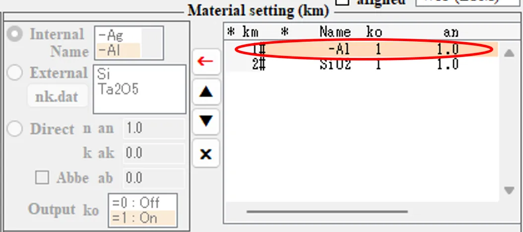
(12) If you click the → button in (9), the editing result will be overwritten.
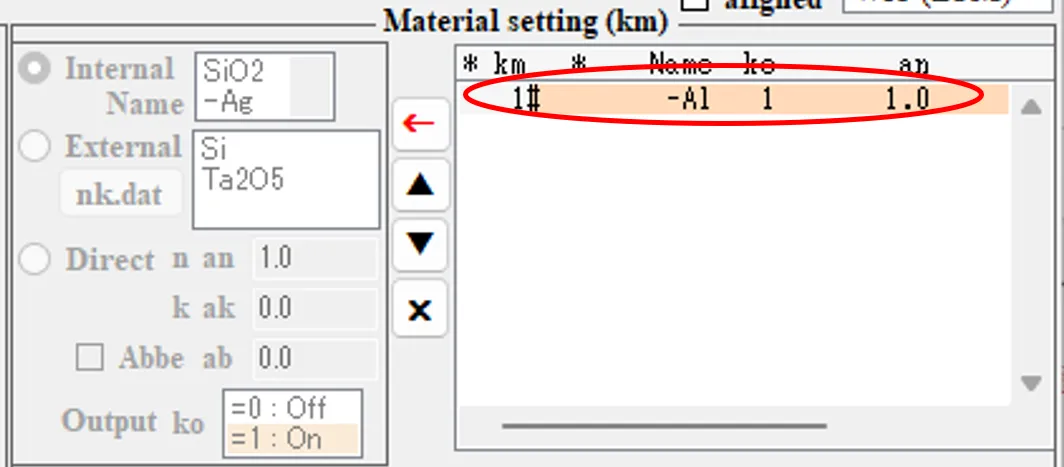
(13) If you click the ↳ button in (9), the editing result will be inserted on the lower side.
● First, in the procedure (1) - (6) below, the background layers of kb = 1 - 27 composed of air (km = 0) are sequentially defined with tk as the film thickness.
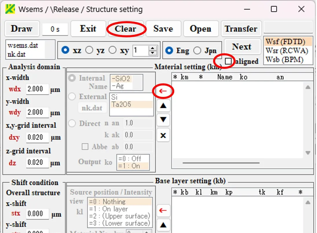
(1) After initializing by clicking the Clear button, uncheck the aligned button and click the ← button in the Material setting field.
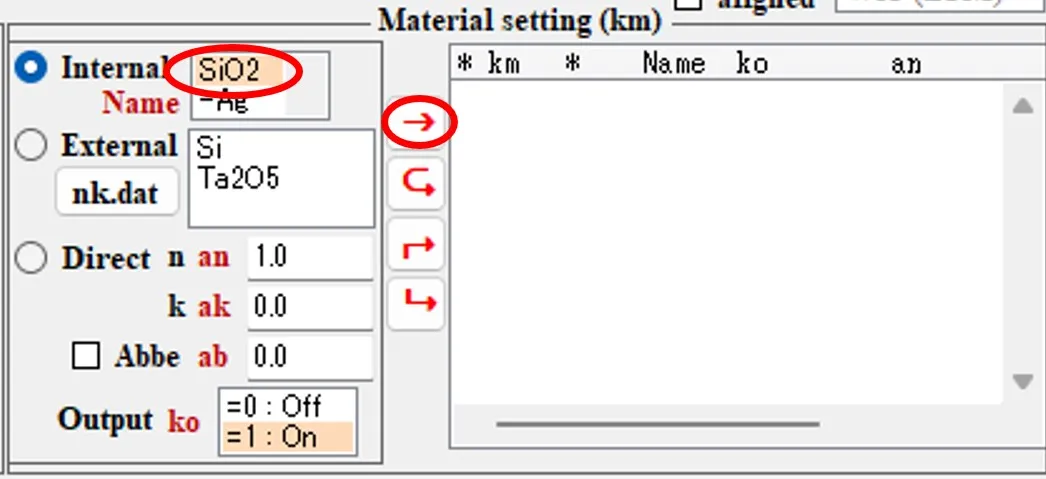
(2) Select 'SiO2' from Internal box. Click the → button to register the first line. Click the ← button in the Base layer setting field.
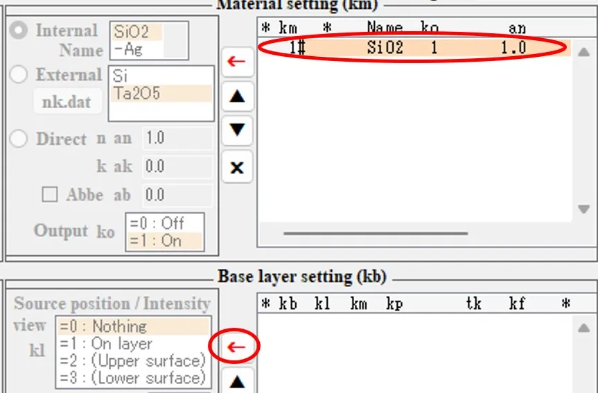
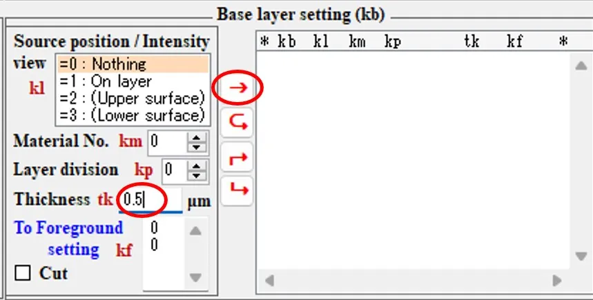
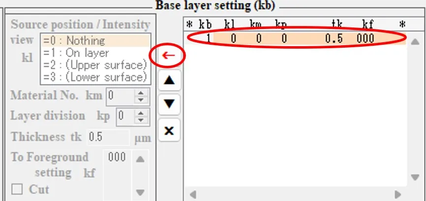
(3) Film thickness tk = 0.5. Click the → button to register the first line. Click the ← button.
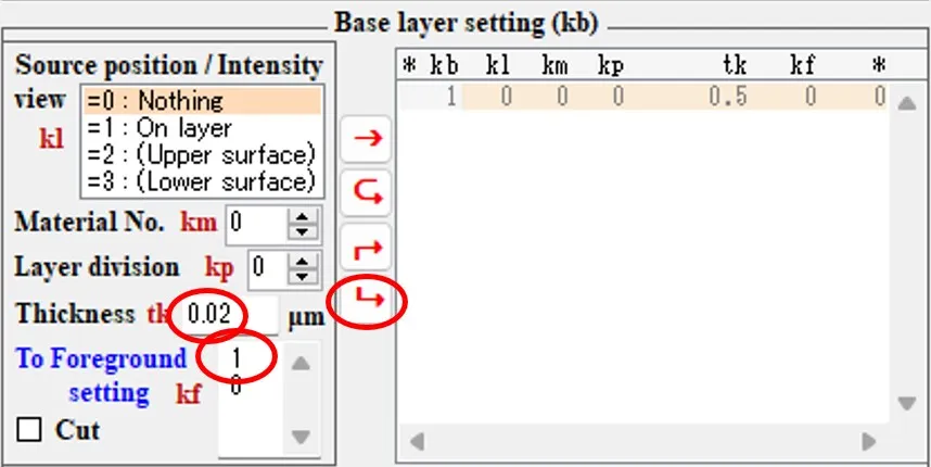
(4) Film thickness tk=0.02, kf=1. Click the ↳ button to register the second line.
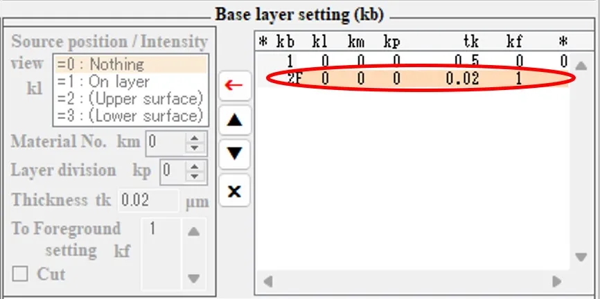
(5) Repeat (3) - (4) while increasing the value of kf by 1 until kf = 25.
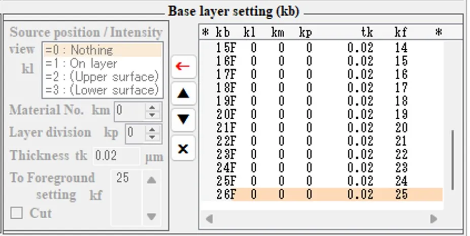
(6) Film thickness tk=2.0, kf=0. Click the ↳ button to register the last row.
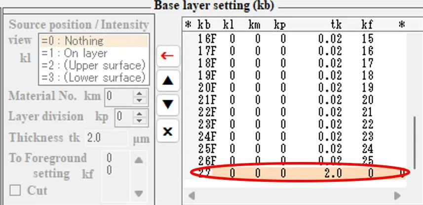
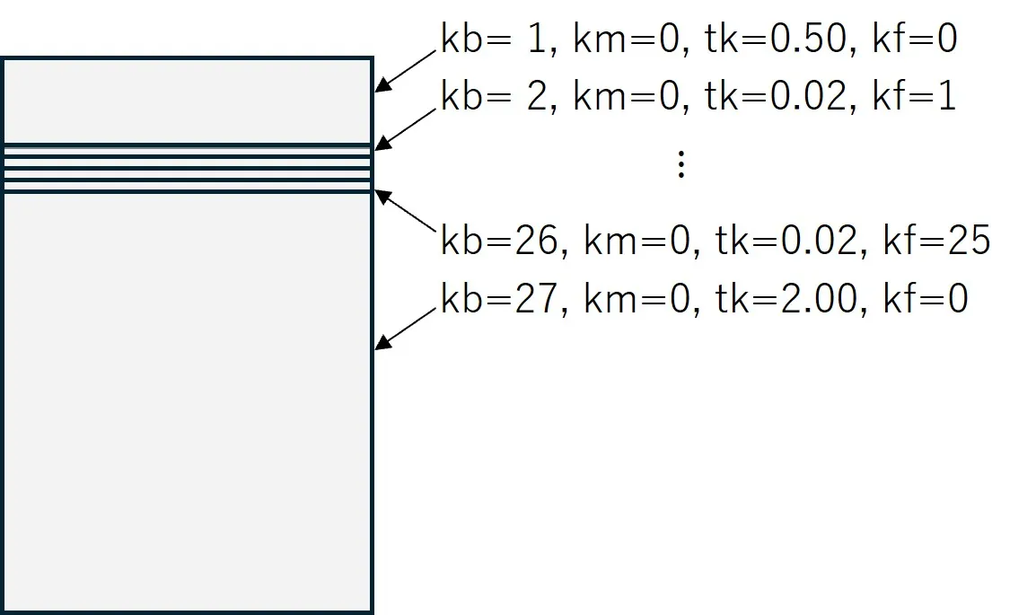
● Next, according to the procedure (7) - (11) below, assign the foreground structure defined in lines 1 - 25 of the Foreground setting field to the background layer for which the value of 1 - 25 is set for kf above.
(7) Click the ← button in the Foreground setting field.
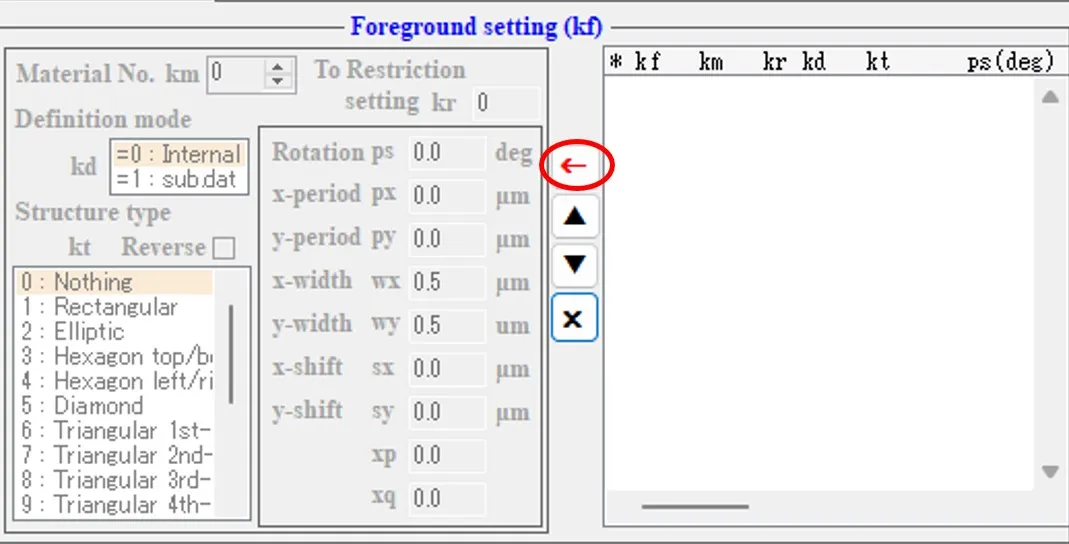
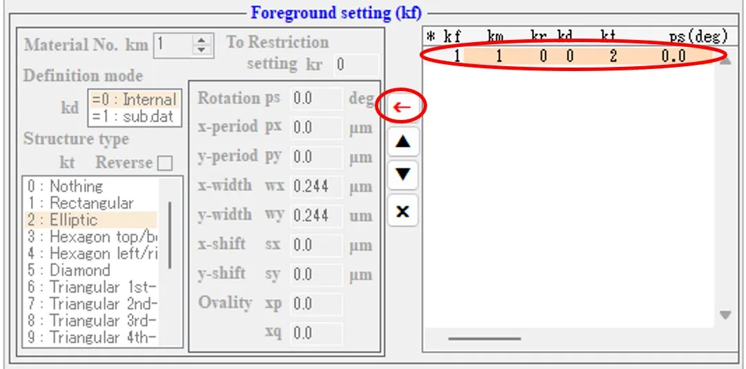
(8) km=1, kd=0, kt=2, px=py=0.0, wx=wy=0.244, sx=sy=0.0. Click the → button to register the first line. It is a foreground structure corresponding to kf = 1 (the background layer for kb = 2).
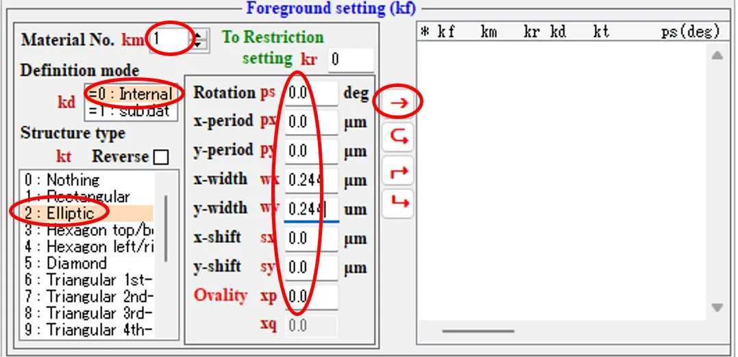
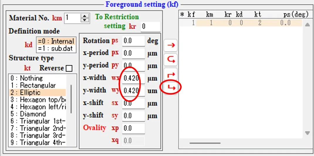
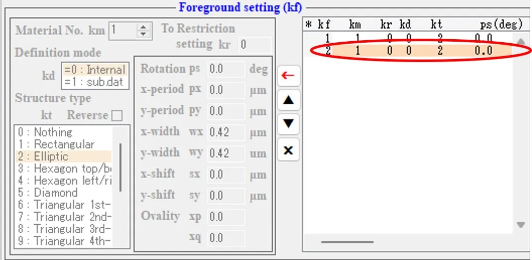
(9) Click the ← button and set wx,wy=0.420. Click the ↳ button to register the second row. It is a foreground structure corresponding to kf = 2 (the background layer for kb = 3 ).
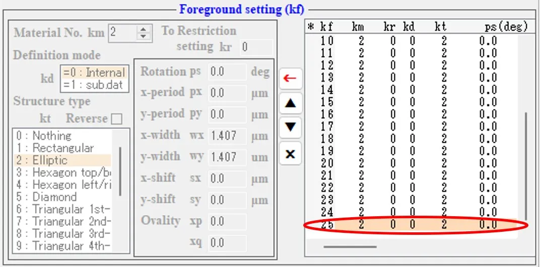
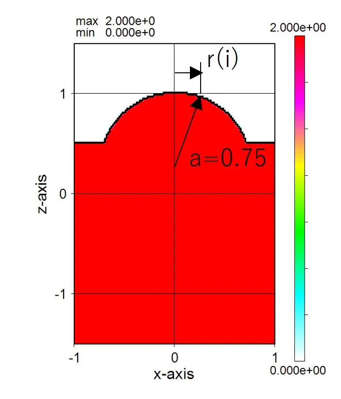
(10) Repeat (8) - (9) as wx=wy=2*r(i), and set the wx and wy values for the number of rows i sequentially until i becomes 25. where r(i) is a solution of a system of spherical surfaces (z=r(i)^2/2a) and indented surfaces (z=(i-1/2)*dz), which corresponds to the cross-sectional radius. The radius of curvature is a = 0.75 μm, and the step width in the z direction is dz = 0.02 μm. Specifically, wx (=wy) is 0.244, 0.420, 0.539, 0.633, 0.712, 0.782, 0.844, 0.900, 0.951, 0.998, 1.041, 1.081, 1.118, 1.153, 1.185, 1.215, 1.243, 1.269, 1.293, 1.316, 1.337, 1.357, 1.375, 1.392, A value of 1.407.

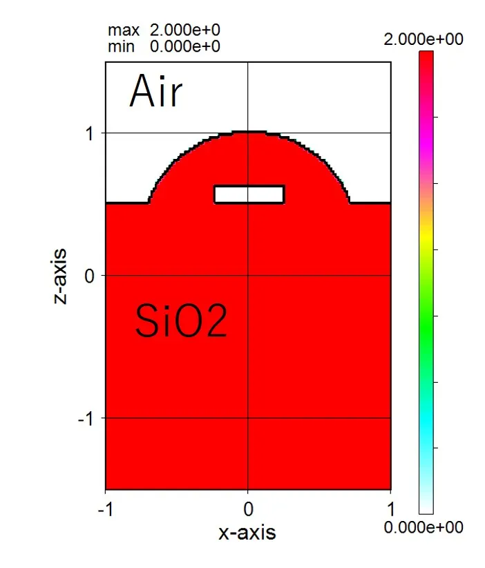
(11) Click the Draw button to draw a cross-sectional view.
● Finally, in the procedure (12) - (14) below, a part of the foreground structure is restricted to form a hollow part.
(12) Change the value kr of the kf=21 - 27 lines in (11) above to kr=1. That is, click on the line kf=21 and click on the ← button.
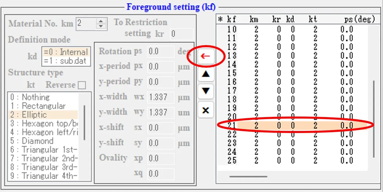
(13) Set kr=1 and click the → button to change the value kr of the line kf=21 to kr=1.
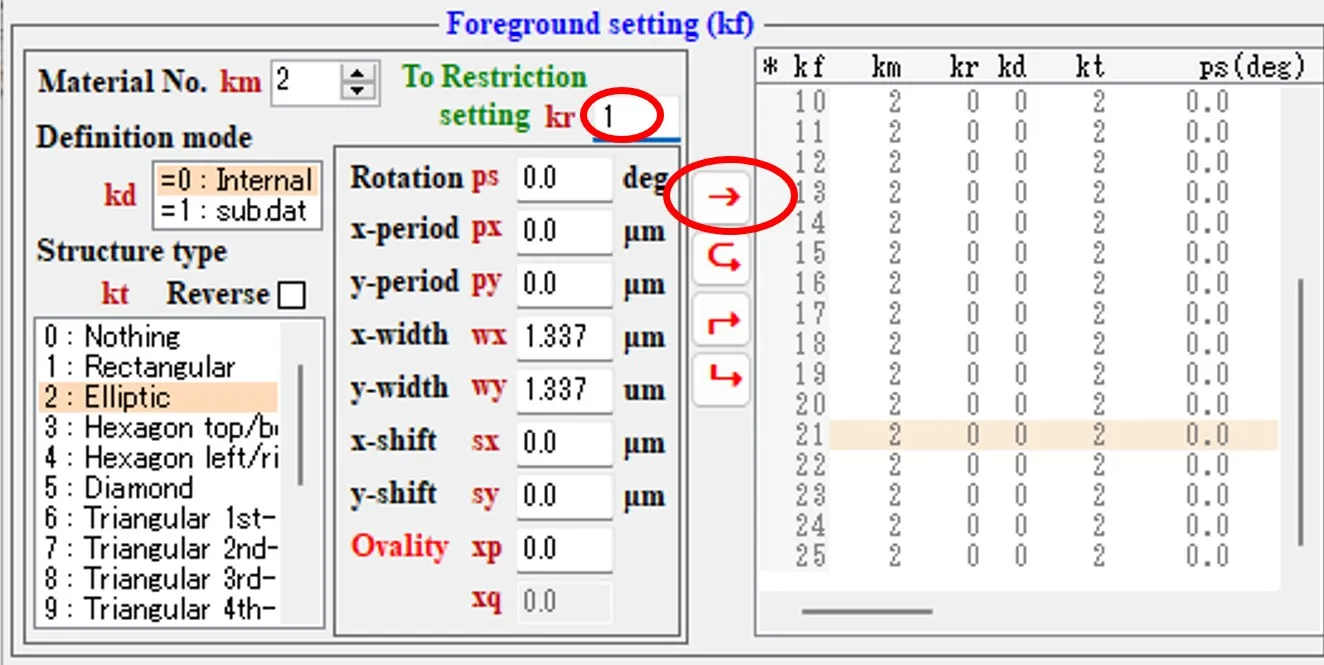
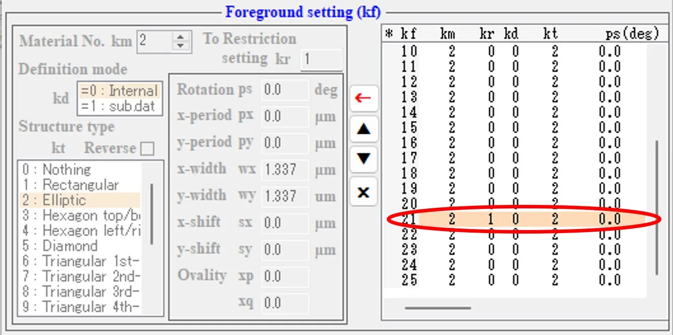
(14) Repeat steps (12) and (13) for lines kf=22 - 25 and change the value kr of the lines kf=21 - 25 to kr=1. As a result, the area restriction defined in the first line of the Restriction setting column is added to the foreground structure of kf = 21 - 25.
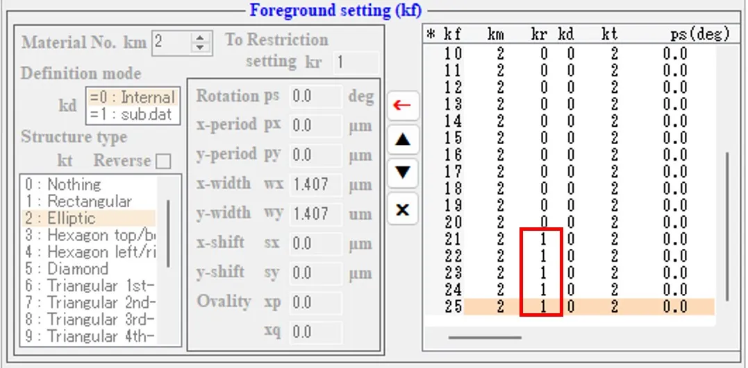
(15) In (12), the following procedure may be used. That is, double-click the wsems.dat in the result file box to open the information window.
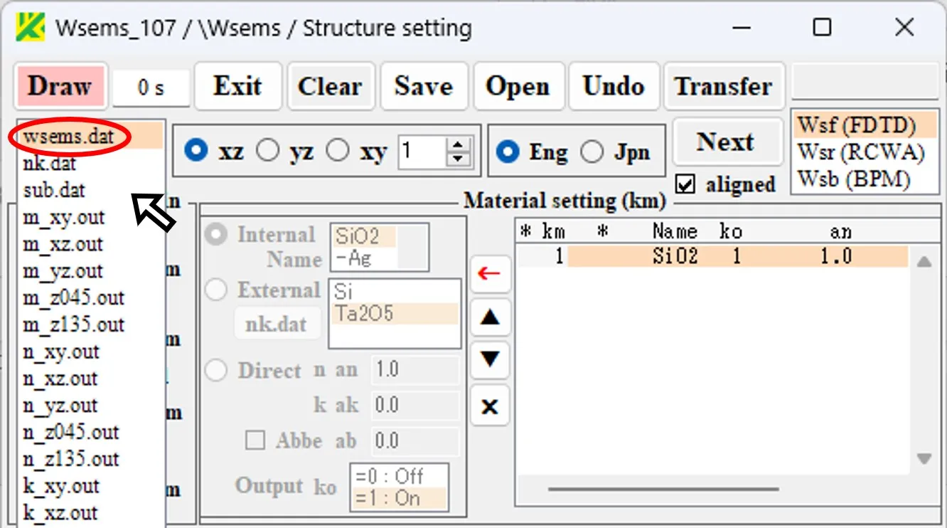
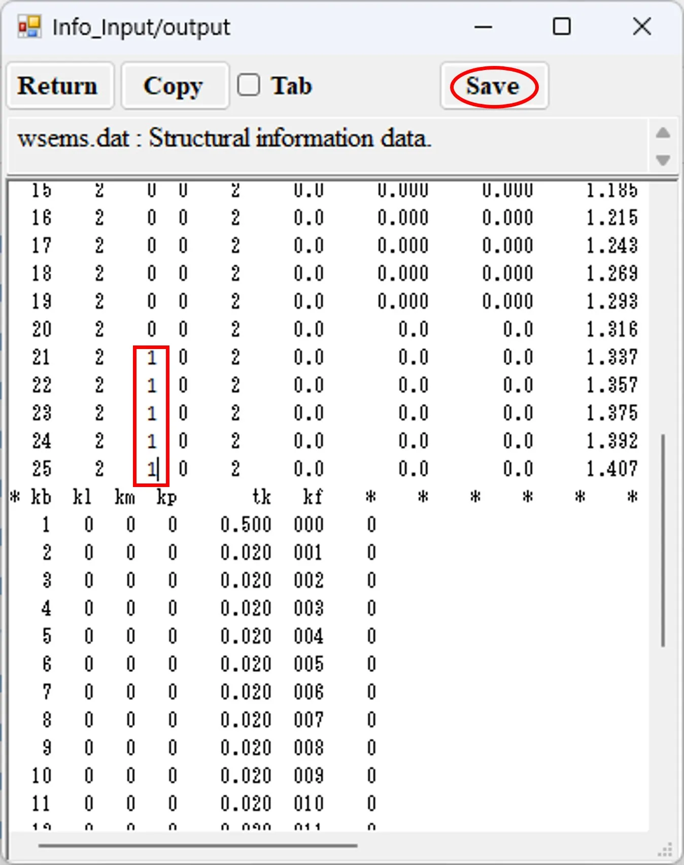
(16) On the information window, change the value kr of the kf=21 - 25 lines to kr=1 and click the Save button to get the state (14).
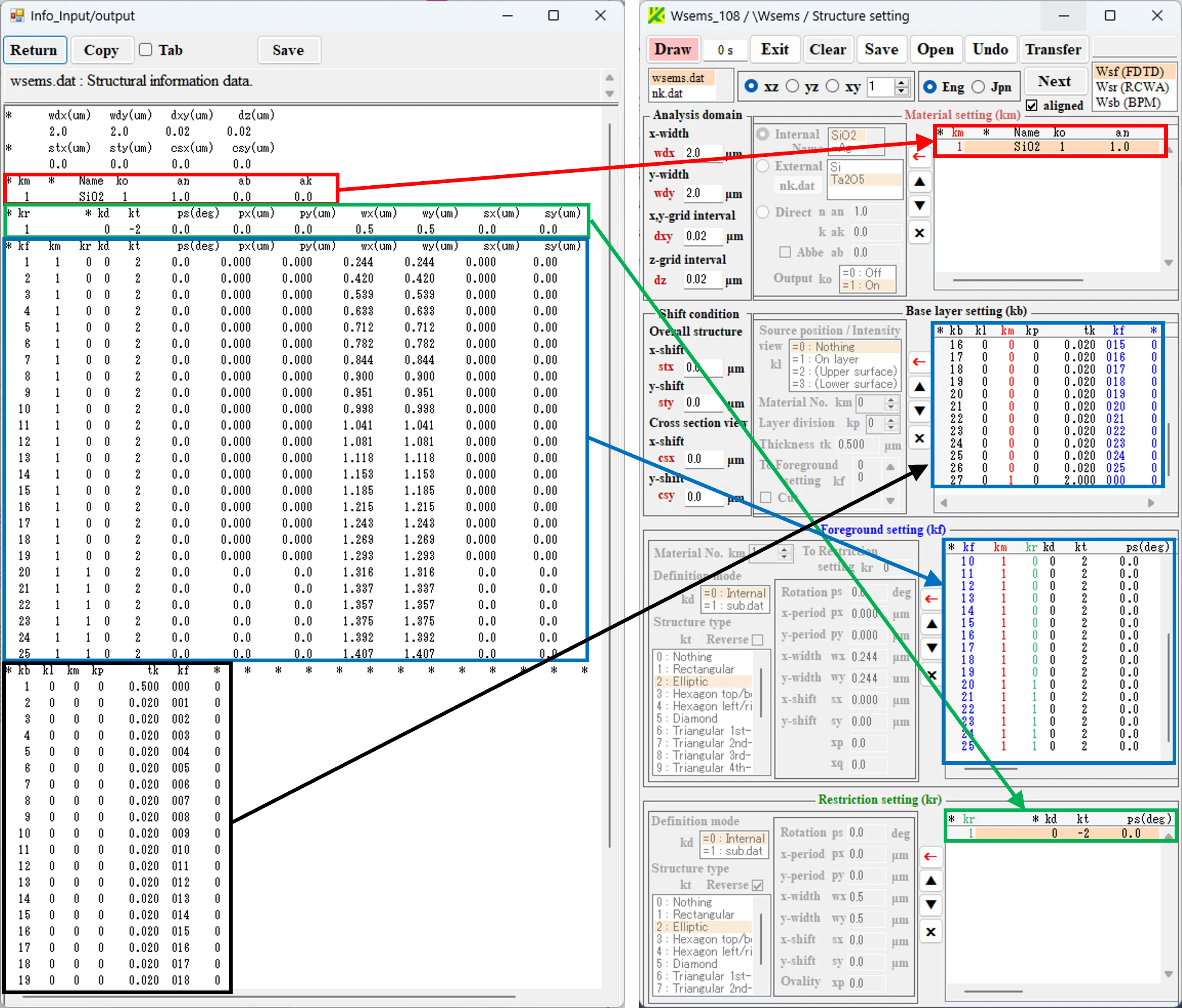
The correspondence between the contents of wsems.dat and the Structure setting window is as follows.
(17) Back to the story, click the ← button in the Restriction setting field. Check the Reverse box and set px=py=0.0, wx=wy=0.50, sx=sy=0.0. Click the → button to register the first row.
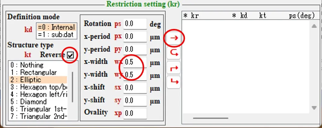
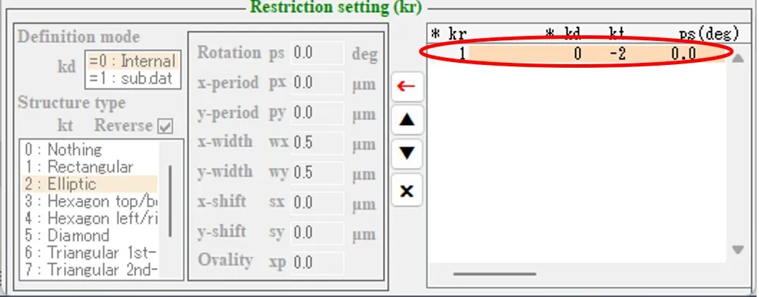
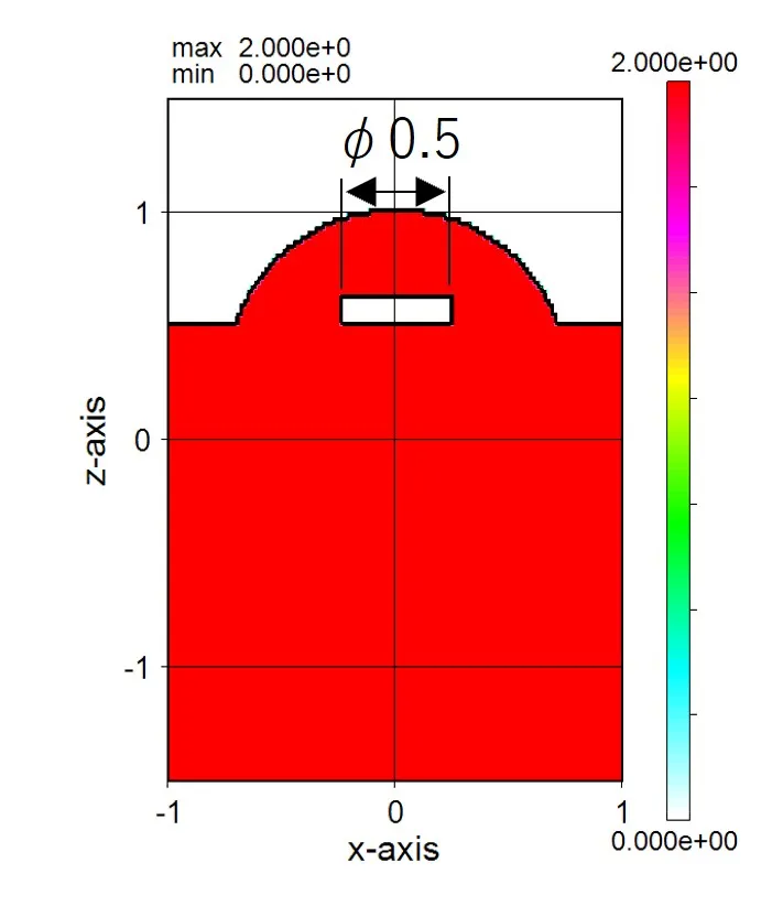
(18) Click the Draw button to draw a cross-sectional view. Since the Reverse box is checked, the foreground structure for kf=21 - 27 is limited to the outside of the circle, and the inside of the circle is hollow.
(19) The Structure setting window has the color coding for the numbers in the registration list, and you can check which field they refer to (Ws_soft_108.zip or later).
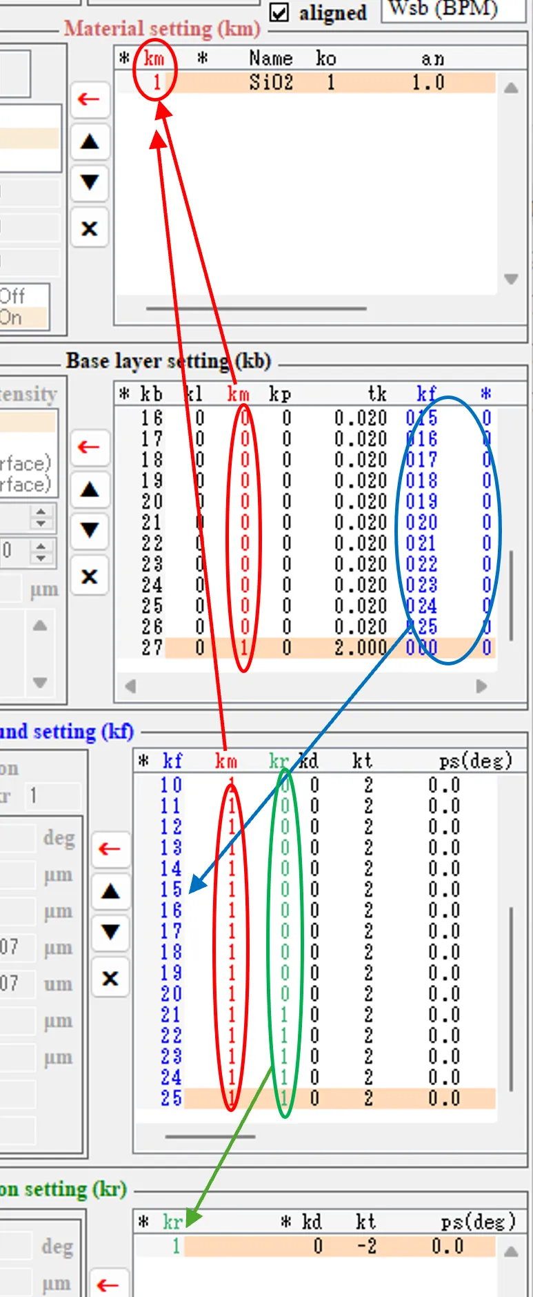
(20) When the aligned box is checked, the reference number correspondence is maintained even if the order of the registration list changes; when the aligned box is unchecked, the reference number correspondence is fixed. In the example below, if -Al is inserted into material list number 1 for the state (19), SiO2 is moved up to number 2, If the aligned box is checked, the km numbers in the Back layer setting and Forground setting fields are also moved up synchronously; if the aligned box is unchecked, they are fixed and remain the same.
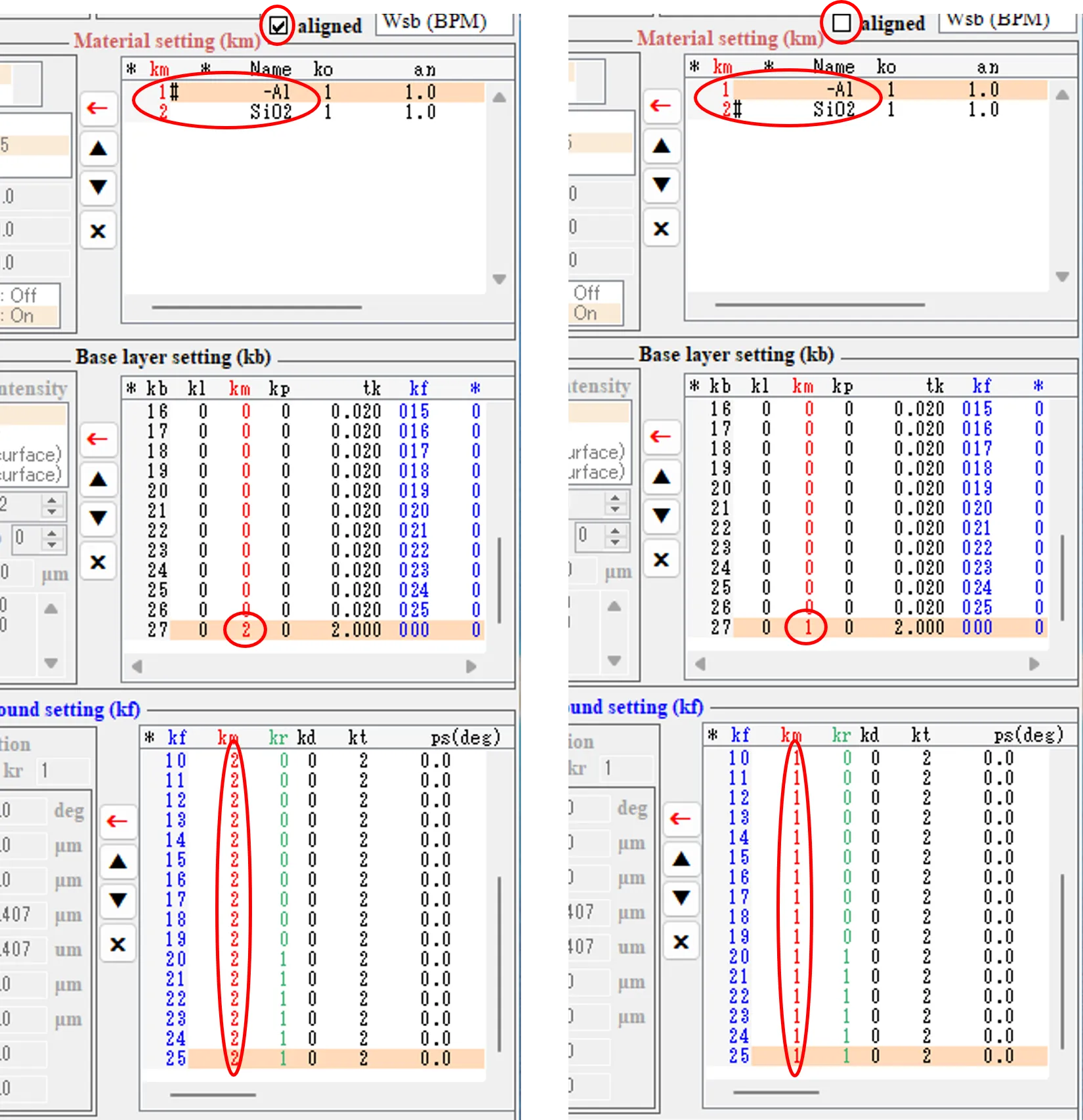
If the aligned box has been operated incorrectly, click on the undo button to recreate the previous state.

● Reference: Alternative method of hollow part formation
The hollow part can be formed without using the Restriction setting field.
(21) Return to the state of (10) above, specify the kf = 25 line in the Foreground setting field, and click the ← button.
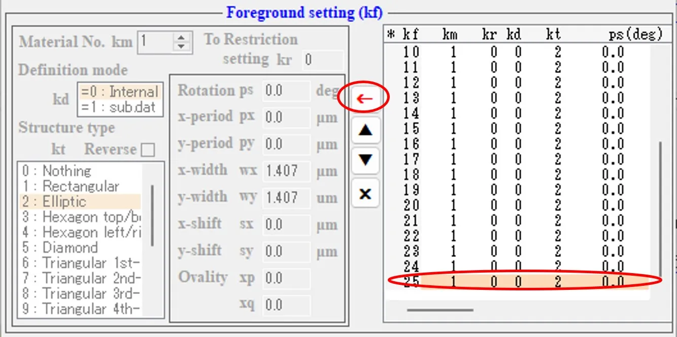
(22) Click the ↳ button as km=0, kd=0(Internal), kt=2(Elliptic), and wx=wy=0.5 to add the line kf=26.
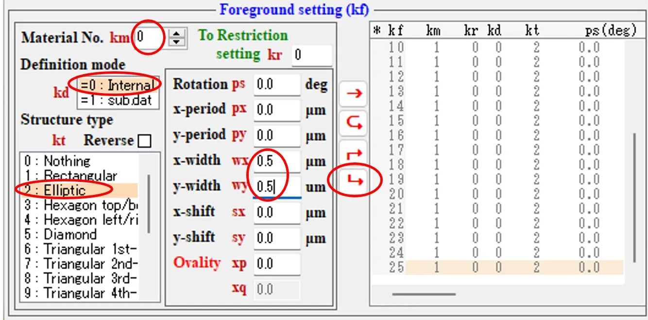
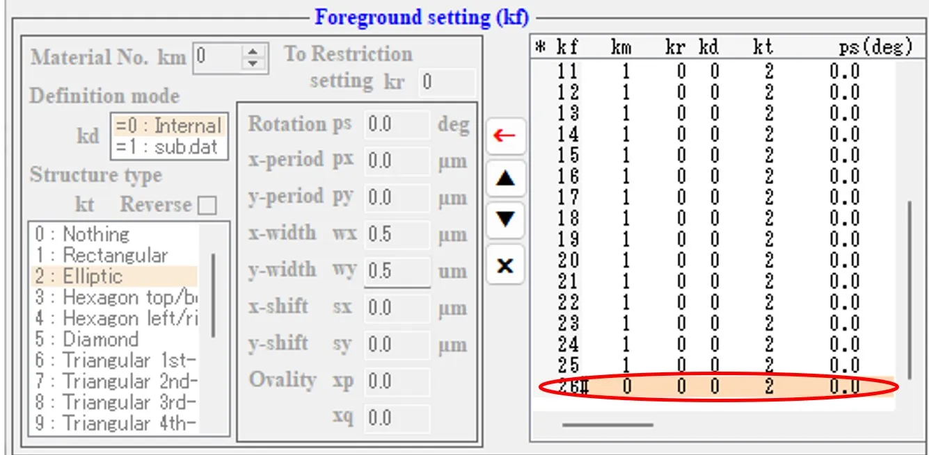
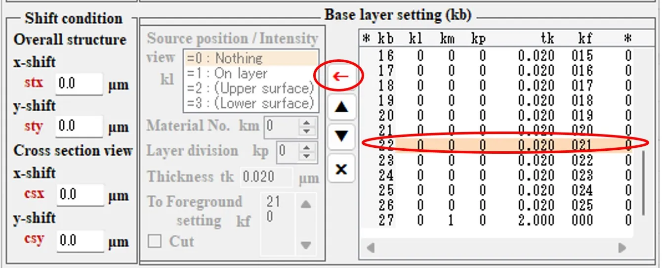
(23) Specify the line of kb = 22 in the Base layer setting field and click the ← button.
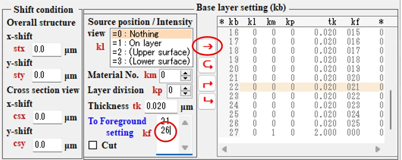
(24) Add "26" to kf and click the button → to change the line of kb=22.
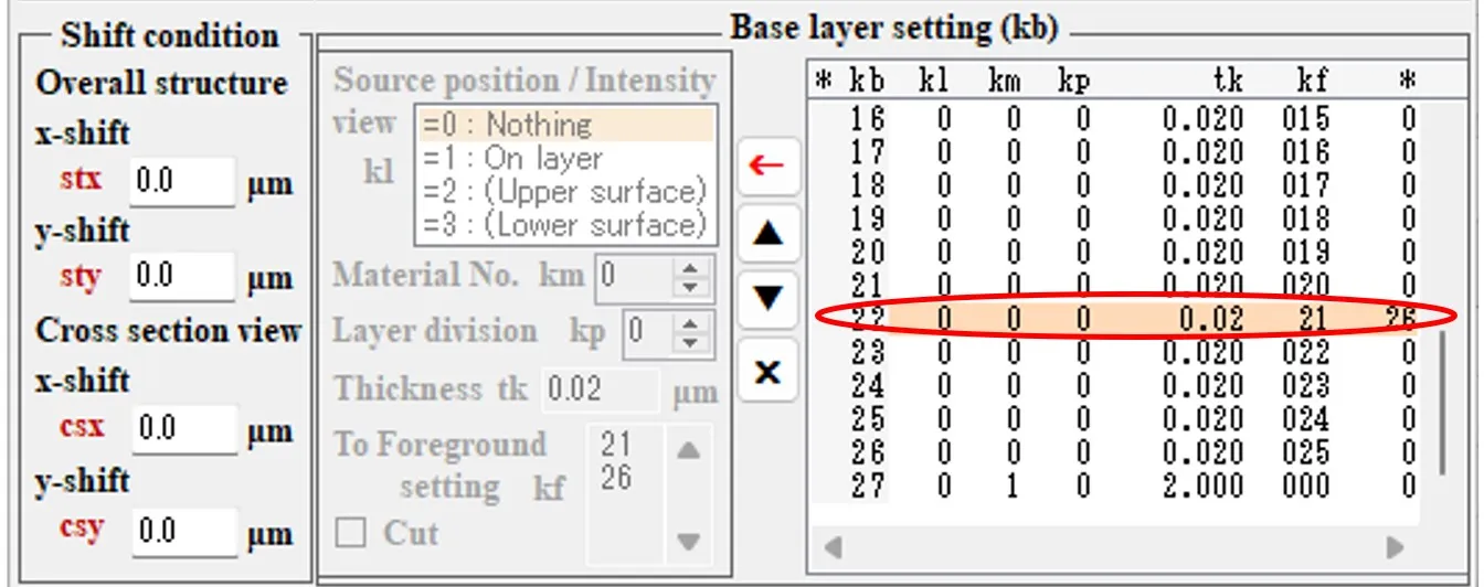
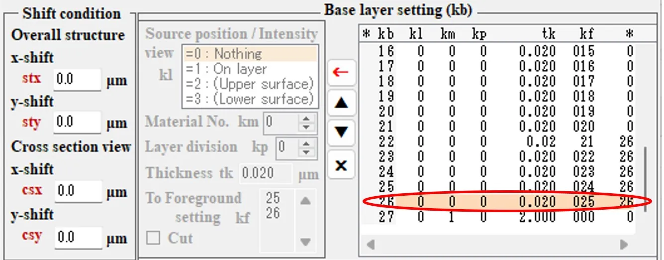
(25) Repeat the same operation as (23) and (24) for lines of kb=23 - 26 and add "26" to kf. In this way, in the lines of kb=22 - 26, kf is set to 25 and 26, and the setting shape of the back (kf=26) is overwritten on the previous setting shape (kf=25). When the Draw button is clicked, it can be confirmed that the same hollow part as (11) is formed.
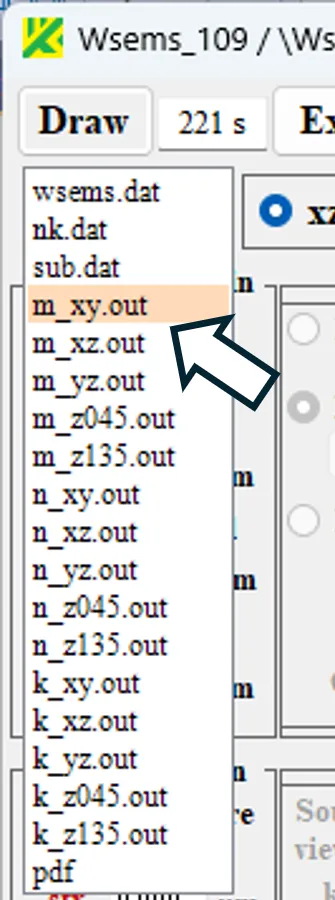
● m_xy.out xy cross-sectional distribution of material numbers.
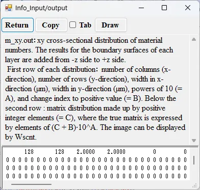
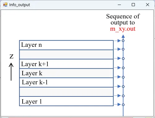
drawing example.
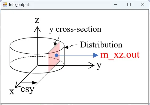
● m_xz.out xz cross-sectional (y = csy) distribution of material numbers.
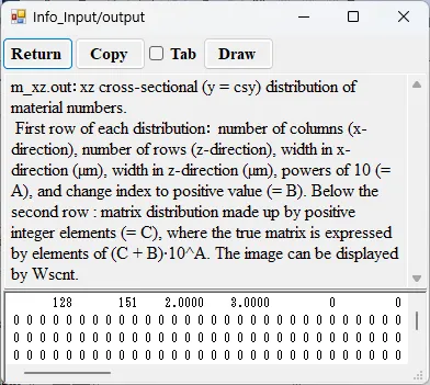
drawing example.

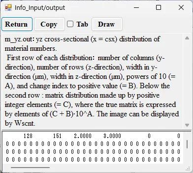
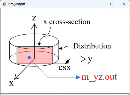
● m_yz.out yz cross-sectional (x = csx) distribution of material numbers.
drawing example.

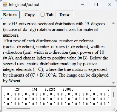
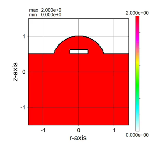
● m_z045.out Cross-sectional distribution with 45-degrees rotation around z-axis for material numbers.
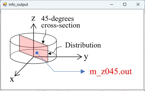
drawing example.
● m_z135.out Cross-sectional distribution with 135-degrees rotation around z-axis for material numbers.
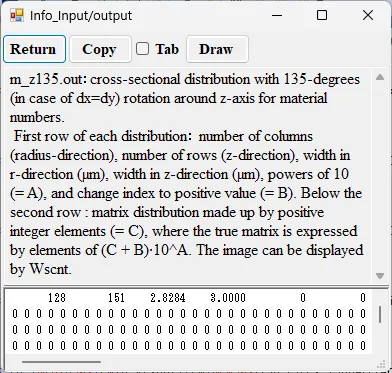
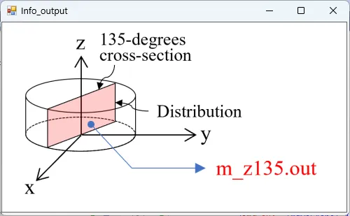
drawing example.
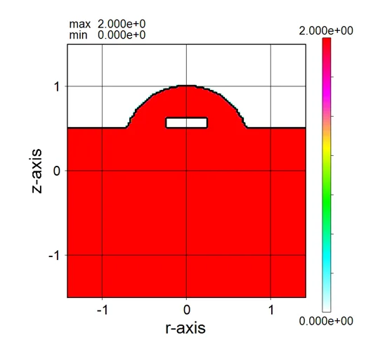
● n_xy.out xy cross-sectional distribution of refractive indexes.
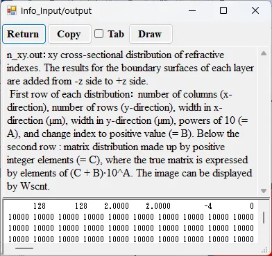
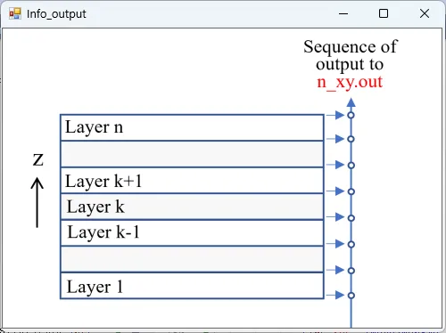
drawing example.
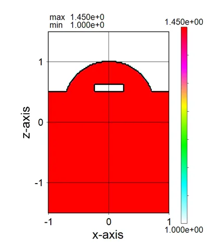
● n_xz.out xz cross-sectional (y = csy) distribution of refractive indexes.
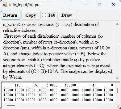
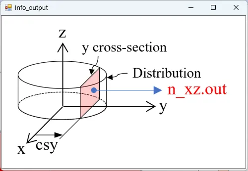
drawing example.
● n_yz.out yz cross-sectional (x = csx) distribution of refractive indexes.
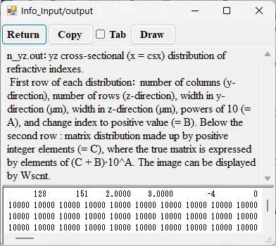

drawing example.

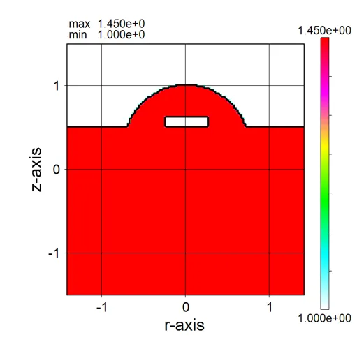
● n_z045.out Cross-sectional distribution with 45-degrees rotation around z-axis for refractive indexes.
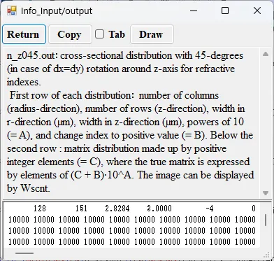
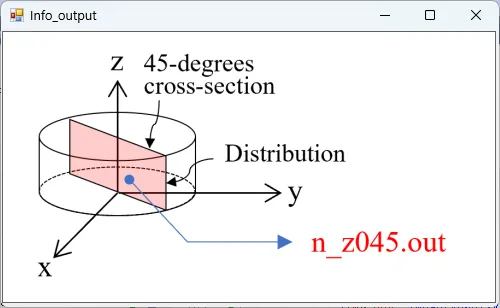
drawing example.
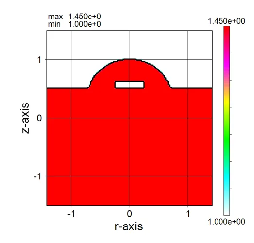
● n_z135.out Cross-sectional distribution with 135-degrees rotation around z-axis for refractive indexes.
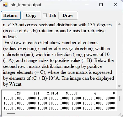

drawing example.
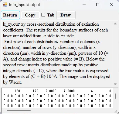
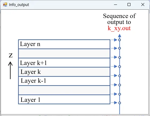
● k_xy.out xy cross-sectional distribution of extinction coefficients.
drawing example.
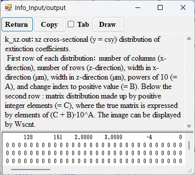
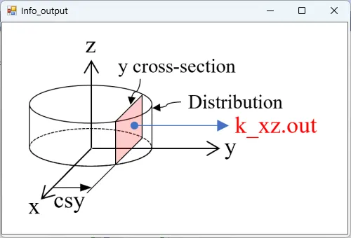
● k_xz.out xz cross-sectional (y = csy) distribution of extinction coefficients.
drawing example.
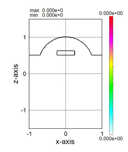
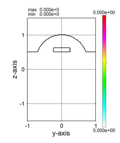
● k_yz.out yz cross-sectional (x = csx) distribution of extinction coefficients.
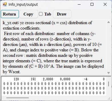
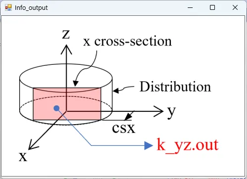
drawing example.
● k_z045.out Cross-sectional distribution with 45-degrees rotation around z-axis for extinction coefficients.
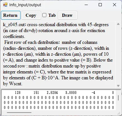

drawing example.

● k_z135.out Cross-sectional distribution with 135-degrees rotation around z-axis for extinction coefficients.
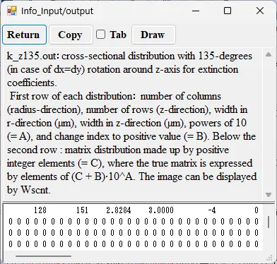
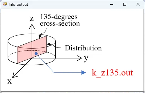
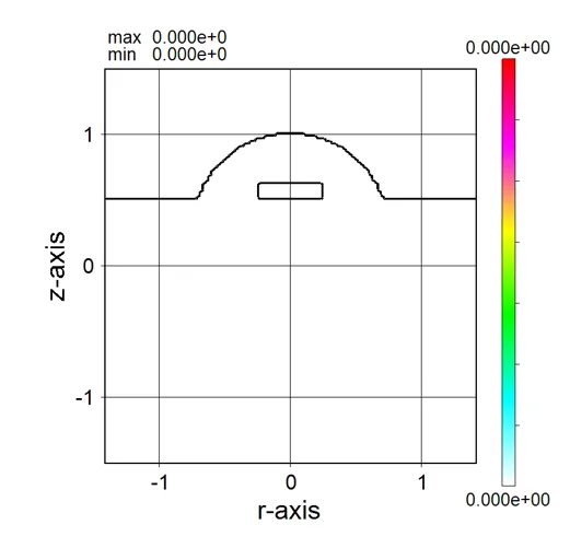
drawing example.
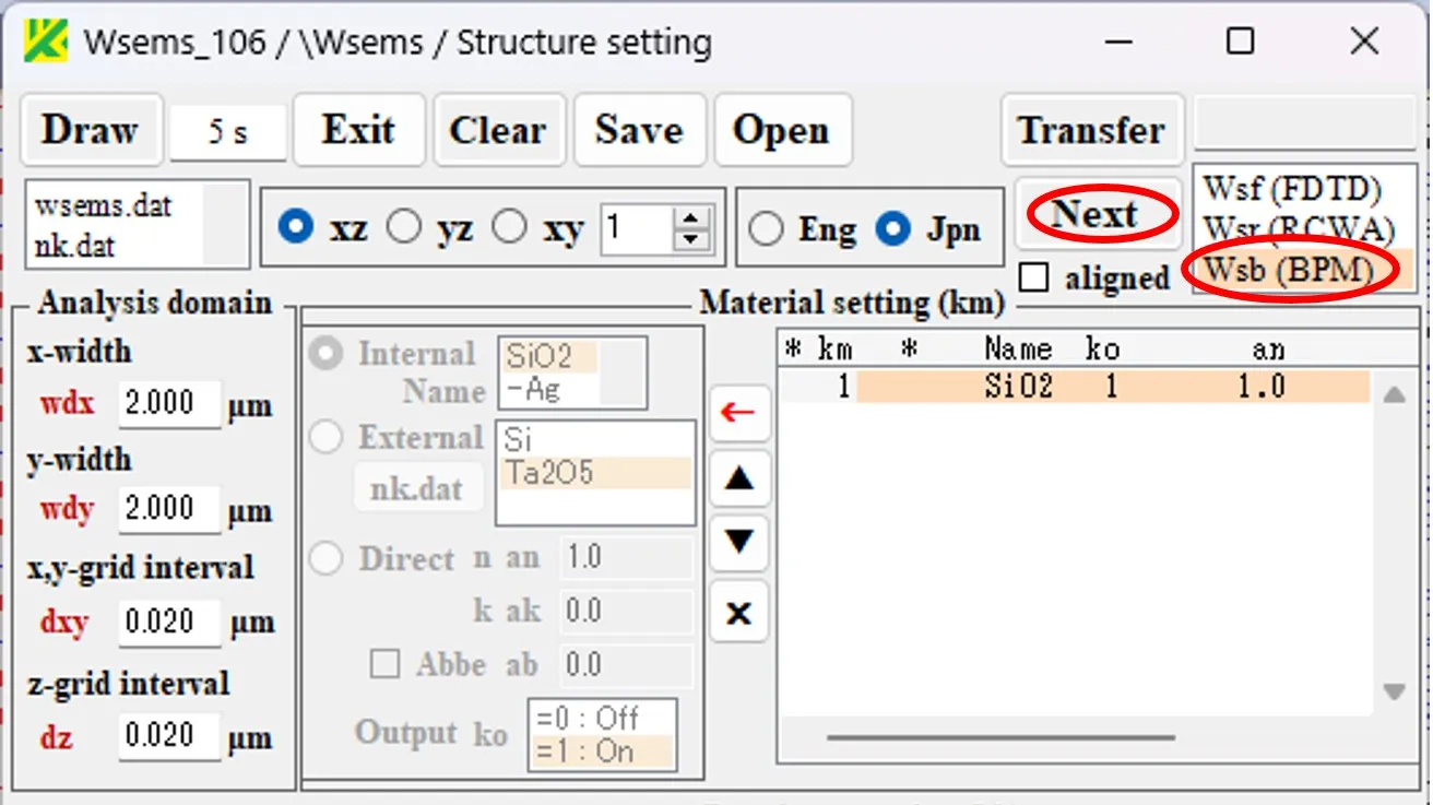
(1) Select 'Wsb(BPM)' and click the Next button to call up the Source setting window.
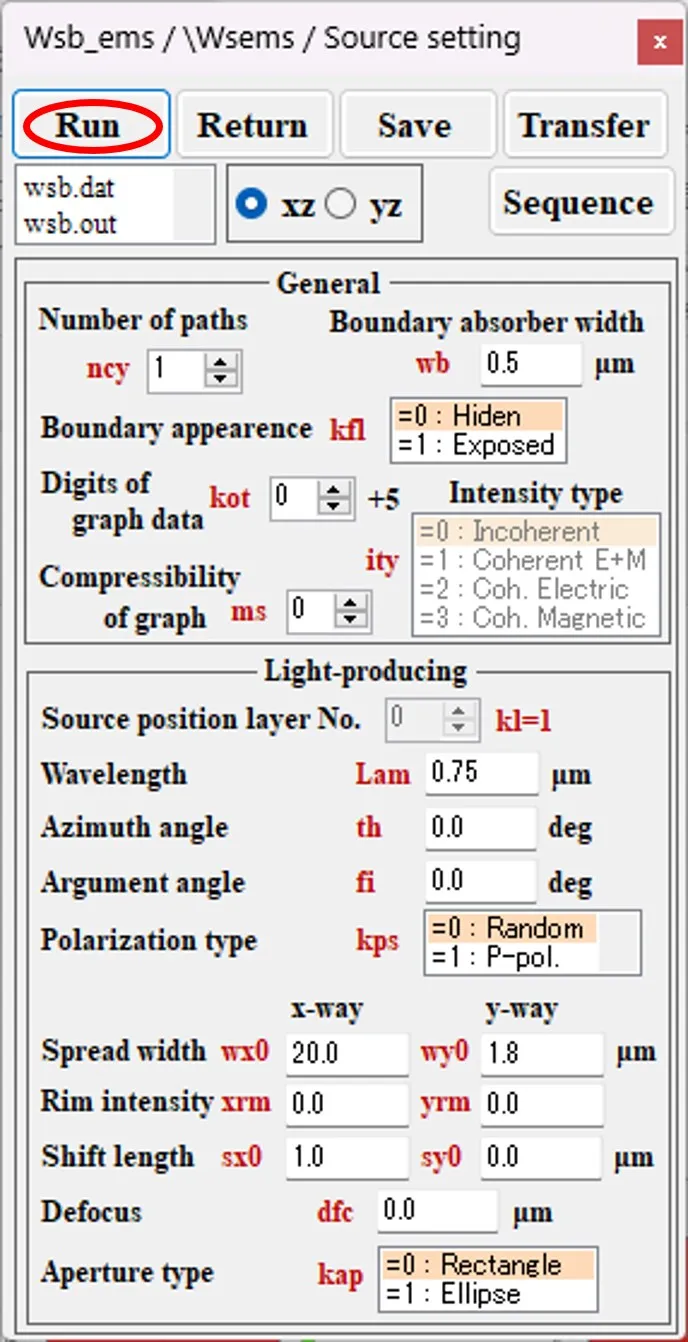
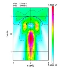
(2) Set the light source conditions and click the Run button. After the wave calculation is completed, Wscnt automatically opens, and the light intensity distribution for the calculation result appears.
● Analyze the results of other calculations.
(3) Double-click 'i_far.out' in the result file box to open the information window.
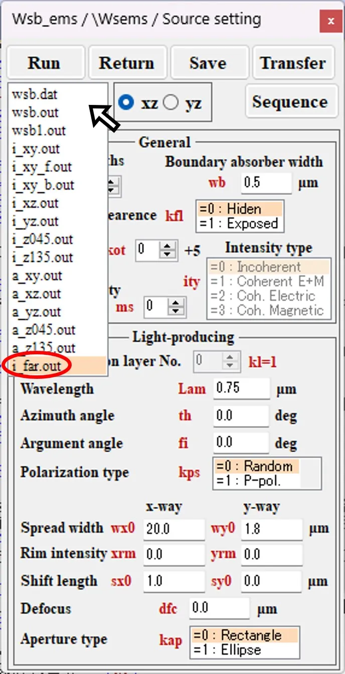
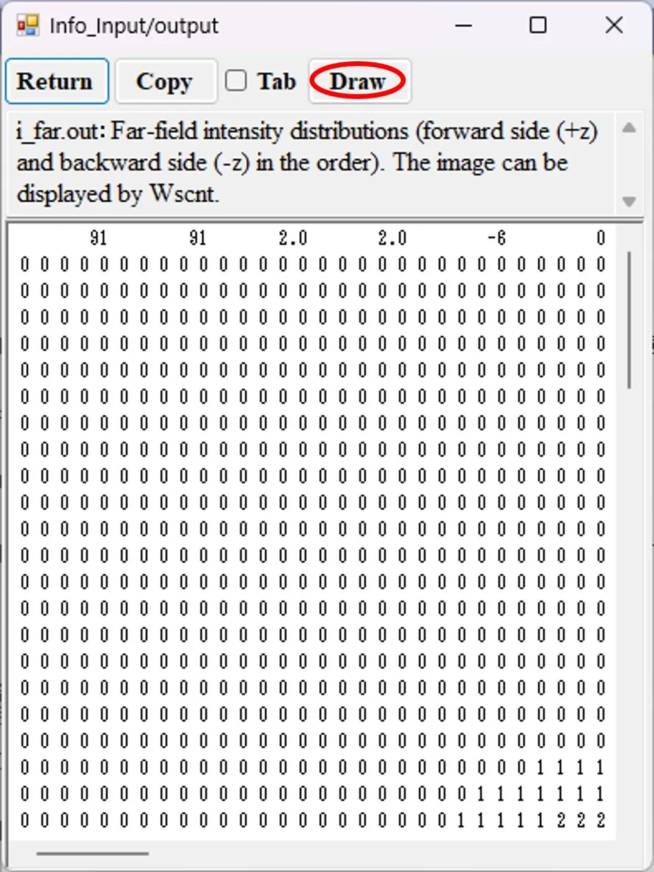
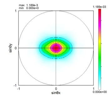
(4) Click the Draw button. Wscnt opens automatically, and the far-field light intensity distribution of the calculation result appears.
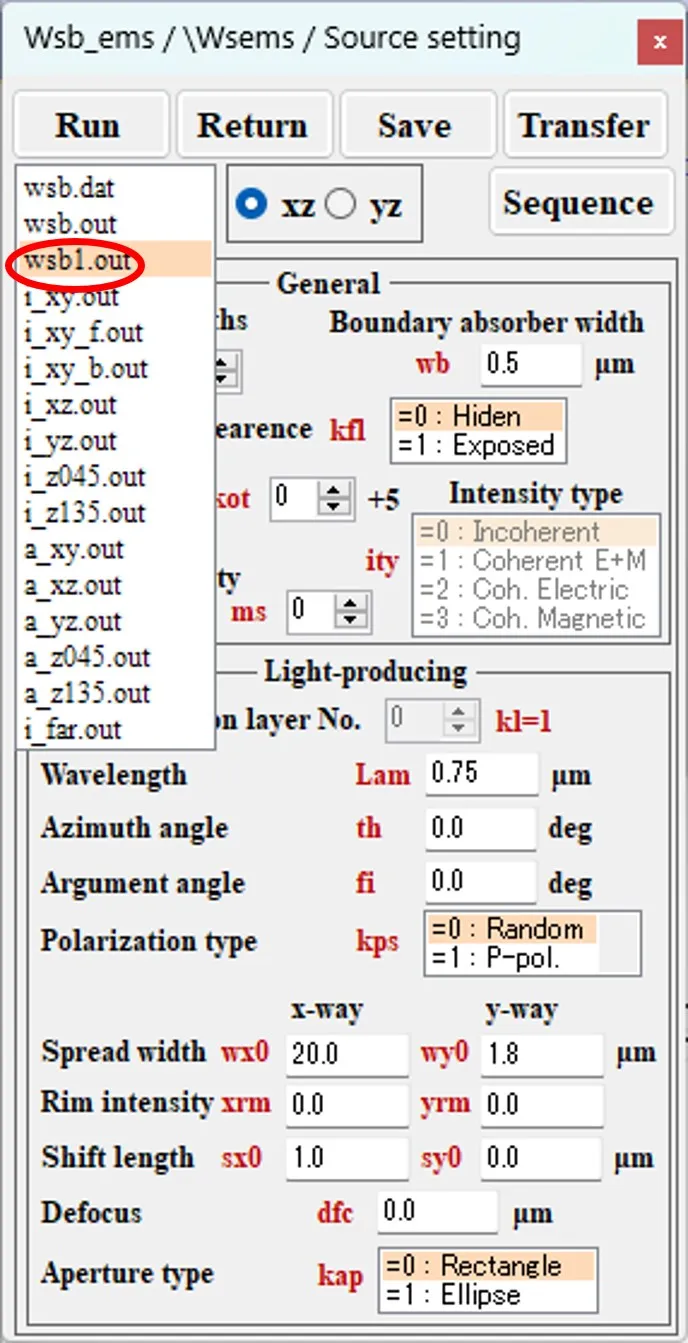
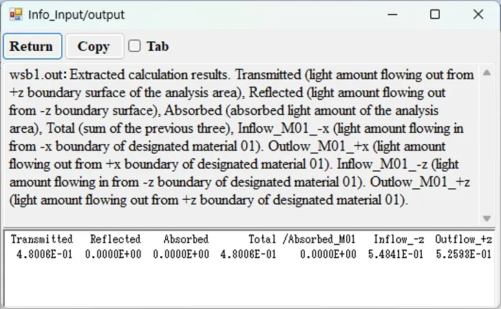
(5) Double-click wsb1.out in the result file box to open the information window. Energy allocation can be analyzed from the contents.
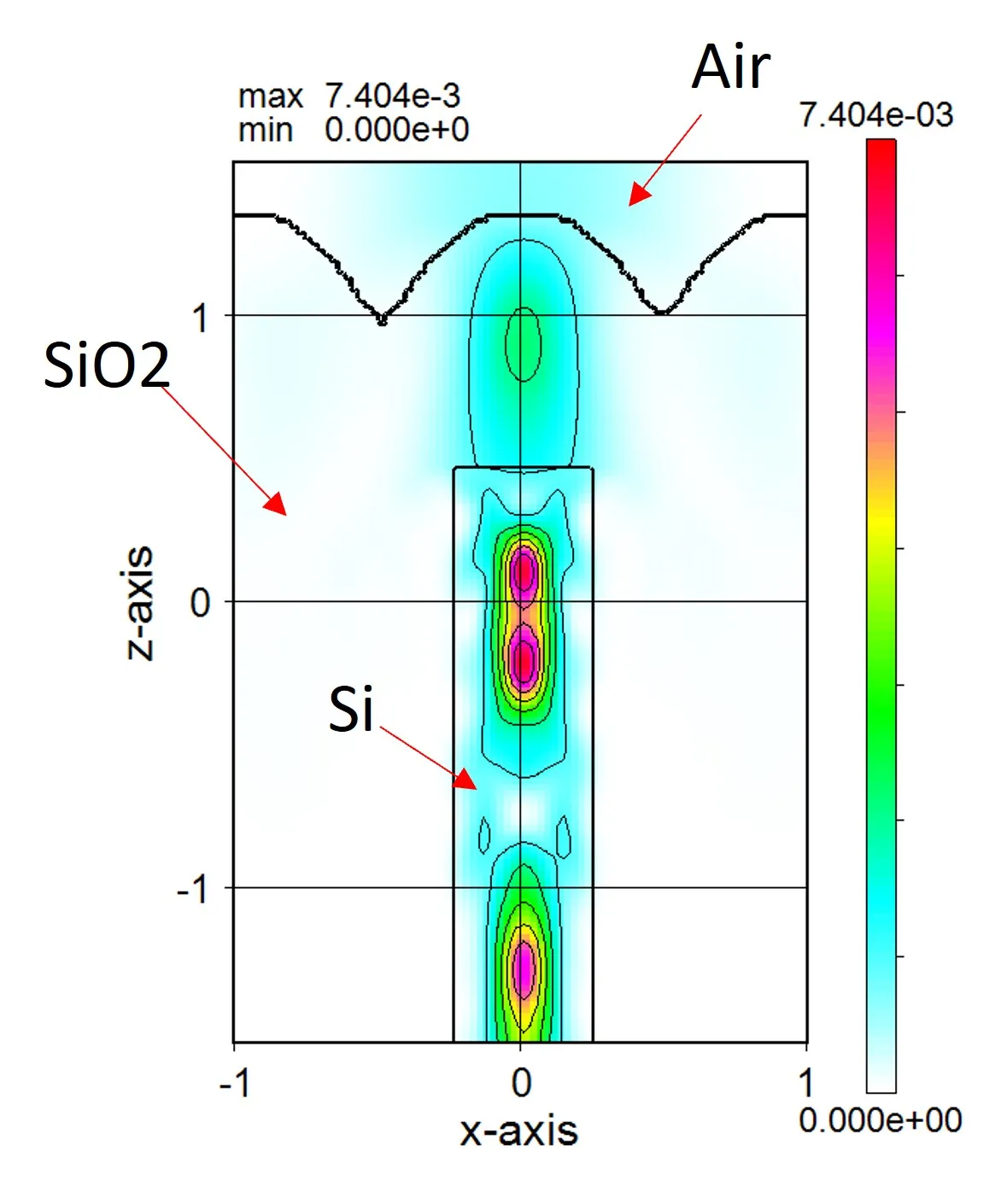
● Since only Air and two types of optical materials (SiO2 and Si) are used, the calculations are performed without restrictions.
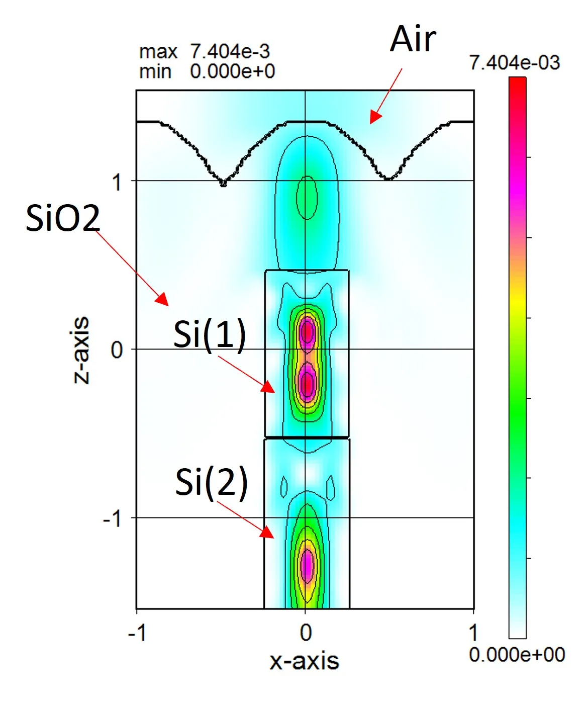
● Since Air and three types of optical materials (SiO2, Si(1) and Si(2)) are used, the calculations are limited and not performed.
(2) If a registered sequrity key (USB dongle) is connected (or MAC address is registered) and the corresponding sup.exe is installed in the folder “Wsems”, calculation starts without any function limitations.
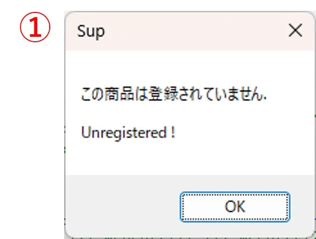
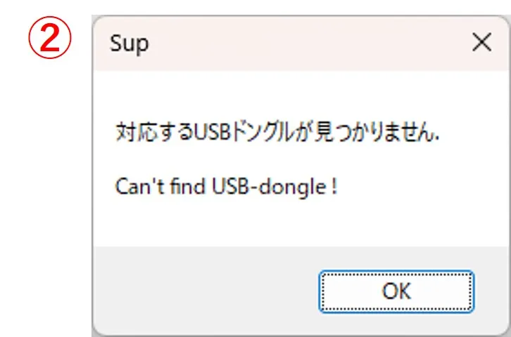
(3) If the sup.exe included in the folder “Wsems” does not correspond to the registered key or registered MAC address, the message ① is displayed for 5 seconds. If the sequrity key is not connected, the message ② is displayed for 5 seconds. If it is within the limitation conditions, the calculation is executed even if the messages ① and ② are displayed.
(4) If you want to purchase, contact us in Inquiry
● Material setting by "Internal"
SiO2, -Ag, -Al, -Au, -Be, -Cr, -Cu, -Ni, -Pd, -Pt, -Ti, -W, and -SiO2 are registered. "-" is added to the beginning of the material name to be calculated as a dispersion material for Wsf (FDTD).
(1) After initializing by clicking the Clear button, click the ← button in the Material setting field to move to the edit panel.

(2) Select SiO2 from "Internal". Click the → button to register the first line.


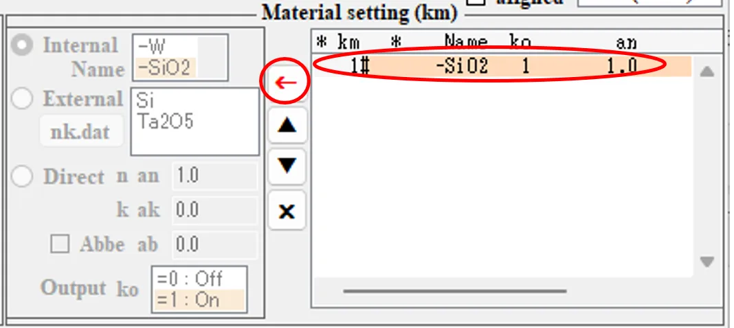
(3) When Wsf (FDTD) is selected, "SiO2" is calculated as a non-dispersed material, and when calculates as a dispersed material, "-SiO2" must be selected (on the other hand, in Wsr and Wsb, there is no distinction between dispersion and non-dispersion, so the "-" at the beginning of the material name is ignored). Here, click the ← button in the Base setting field and select -SiO2 of Internal.
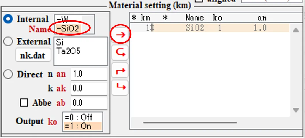
(4) Click the → button to rewrite and register the first line. When handling dispersed materials in Wsf (FDTD), the Courant index "crn" of the Source setting window must be set to 0.9 or less.
● Material setting by "External"
\Samples\Editing the nk.dat based on the nk_data.xlsx references.
(5) Click the ← button to move to the edit panel.
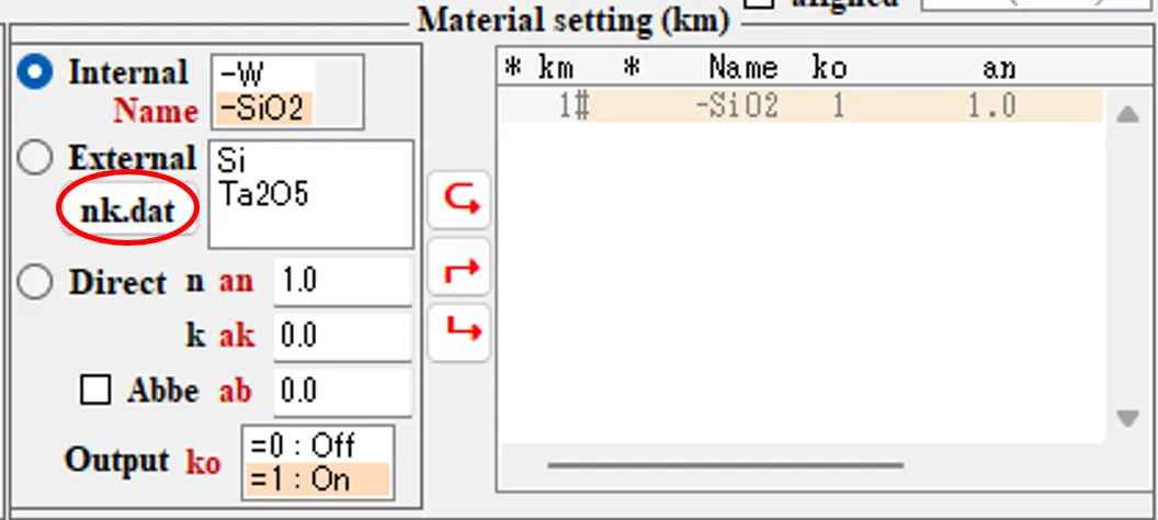
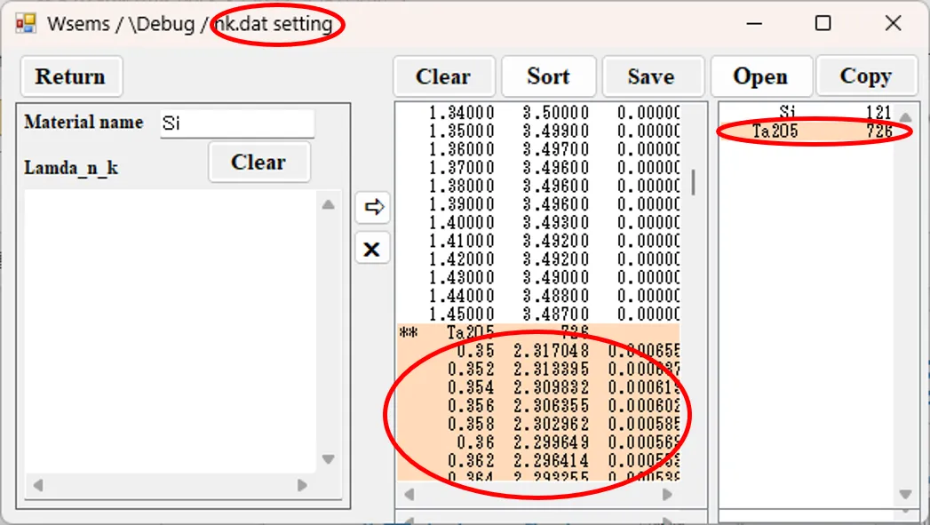
(6) When you click the nk.dat button, the External button is checked and the nk.dat setting window appears. When you click the material name (Ta2O5) in the rightmost box, the dispersion data (wavelength, refractive index, and extinction coefficient columns) for the corresponding material is selected (inverted in blue) in the center box. The same applies when you click on a line with a material name that starts with **, and the dispersion data in the following rows is selected.
(7) Click the × button to delete the material data in the selection.
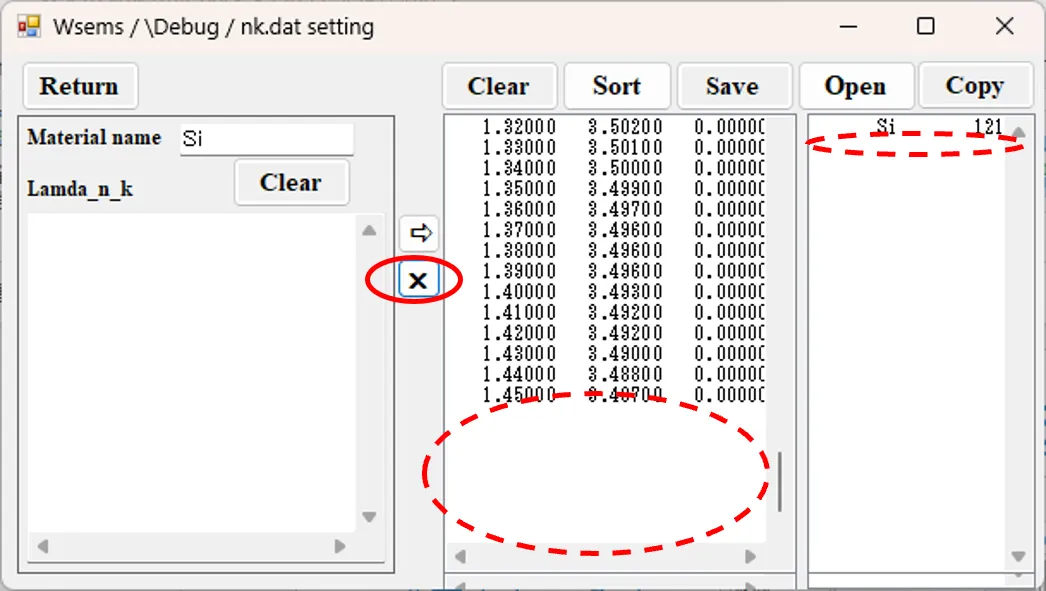
(8) Note: Lines other than ** can be selected individually and can be deleted with the × button.
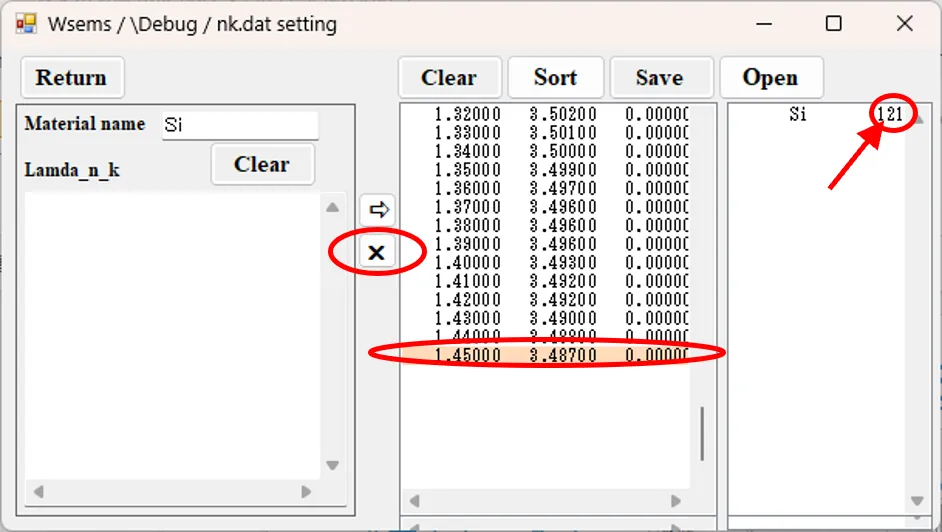
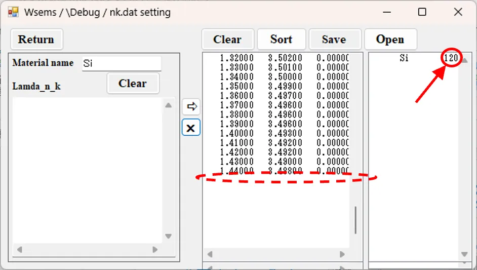
The change in the number of rows due to deletion is reflected in the counter in the upper right.
(9) Return to (7), write Ta2O5 in the Material name box, paste the dispersion data summarized in Excel in the lower box, and click the ⇒ button.
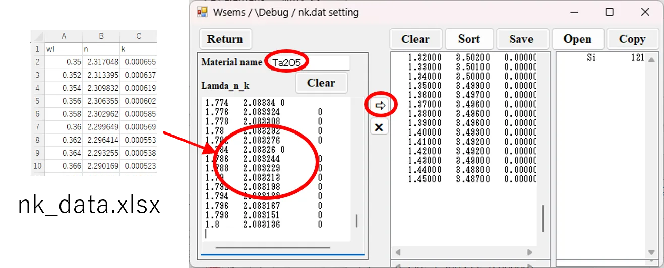
(10) The material name (Ta2O5) and the dispersion data are registered in the list (click the Sort button to arrange the material names in the list).
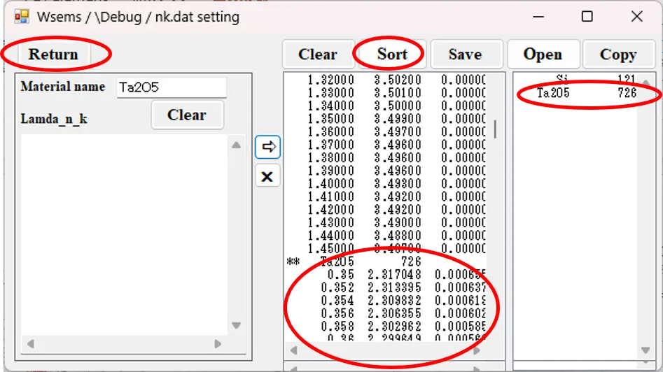
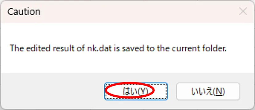
(11) Click the Return button and click "Yes" in the Causion window that appears.
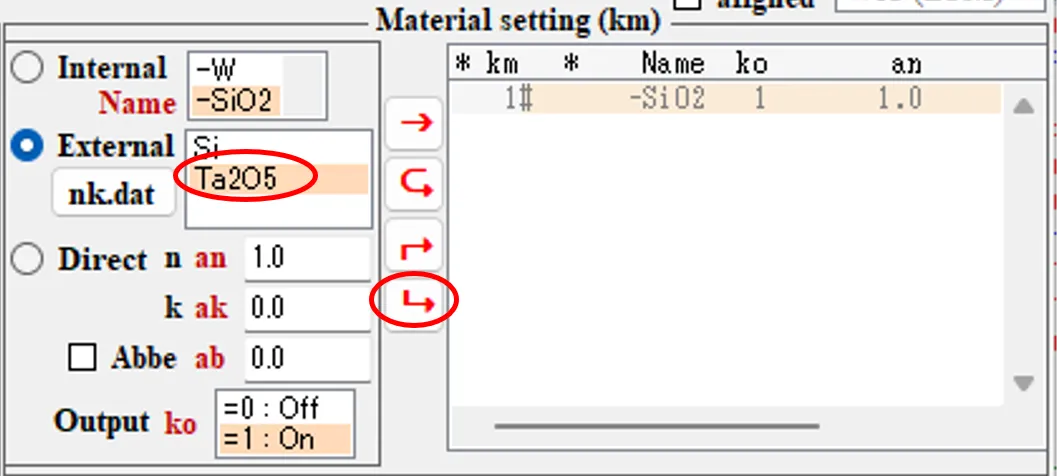
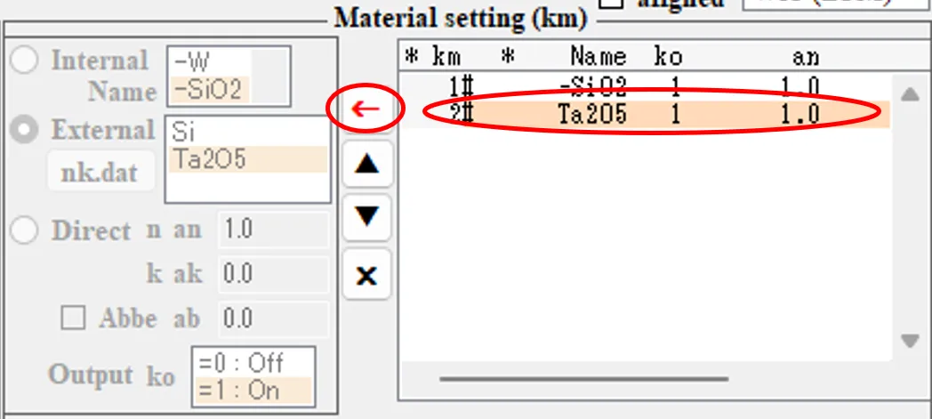
(12) Ta2O5 is registered in the External list. Select this and click the ⮡ button to register the second line. Click the ← button to go to the edit panel.
● Material setting by "Direct"
(13) Click the Direct button. Edit the box on the right of the Direct button (refractive index an = 1.52, extinction coefficient ak = 0.00, Abbe number ab = 30.0 with the checked Abbe box) and click the ⮡ button.
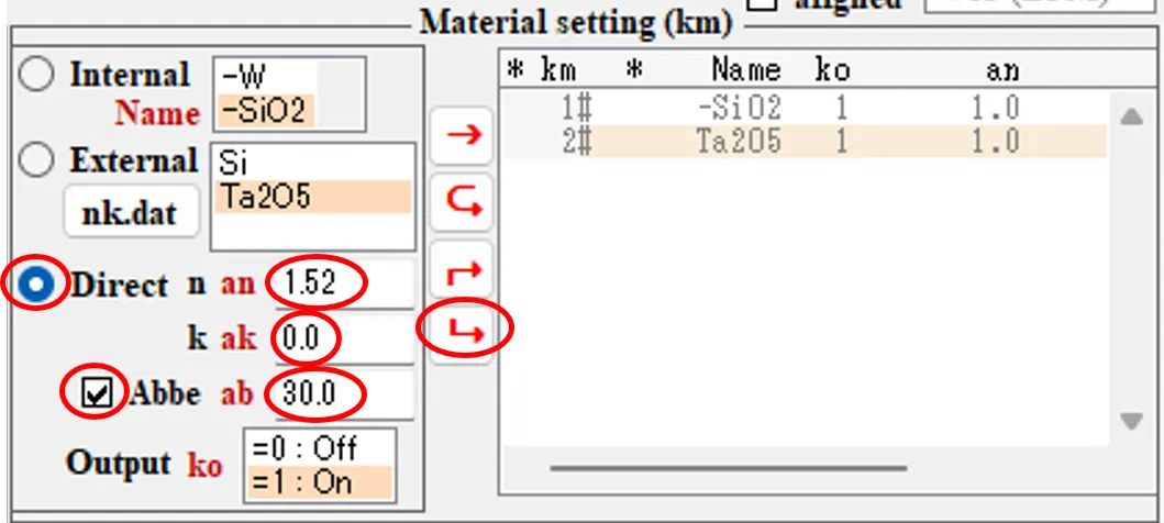
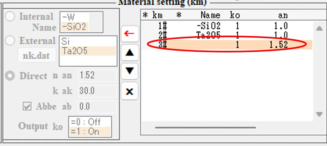
(14) In the third row of the list, the material with n = 1.52 is registered.
● Other ways to desplay the nk_dat setting window
In addition to the methods (5) and (6), there are other ways to call the nk_dat setting window.
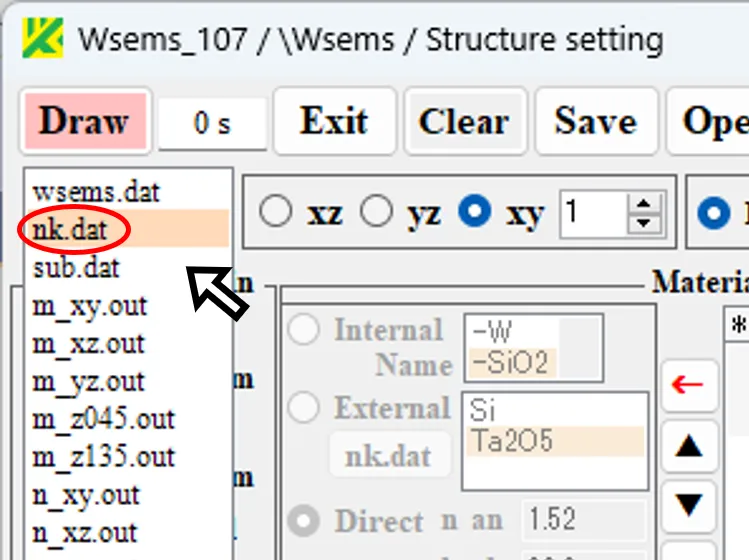
(15) Move the mouse pointer to the result file box on the Source setting window and double-click "nk.dat" in the box to display the information window (Info).
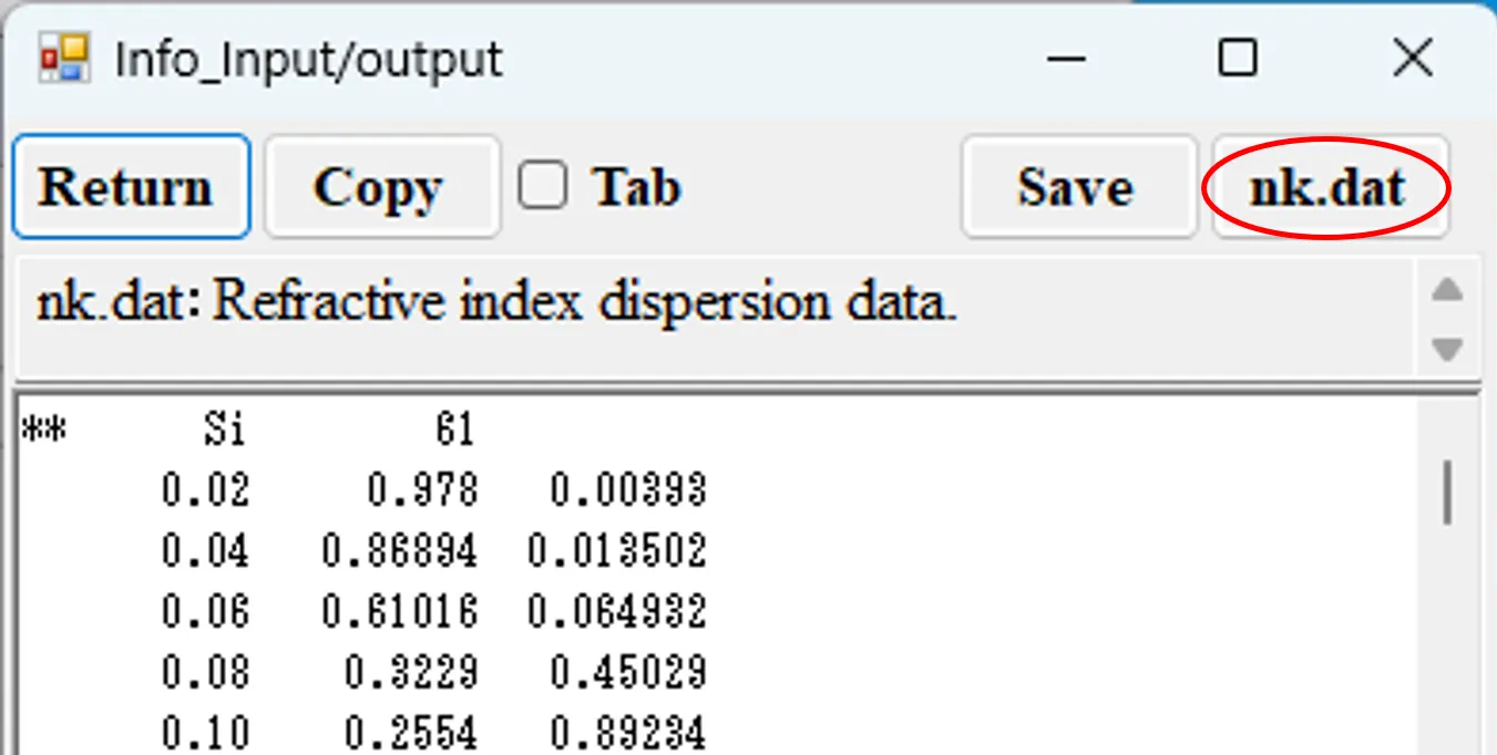
(16) When the nk.dat button on the information window is clicked, the nk.dat setting window as same as (6) appears.
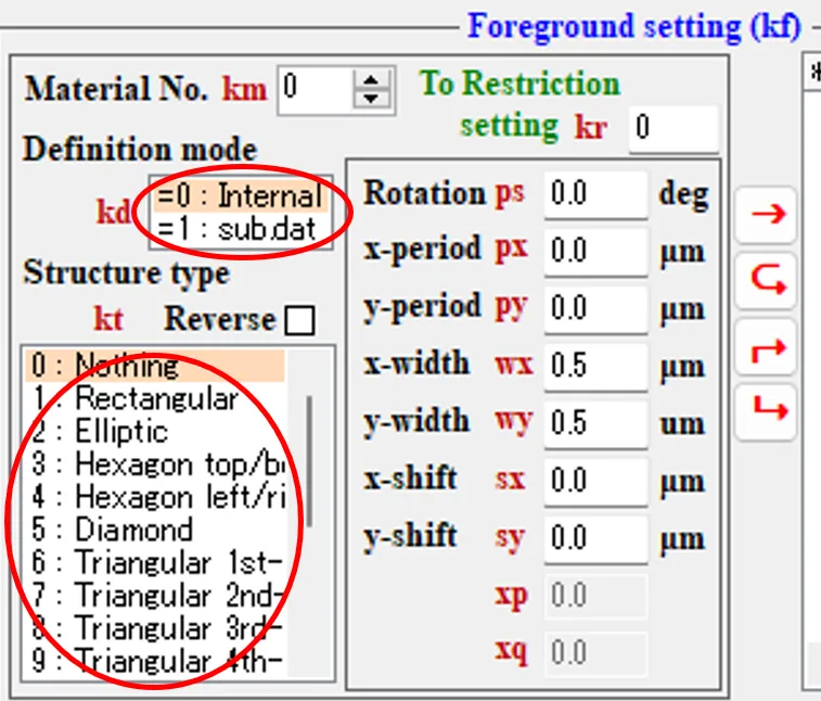
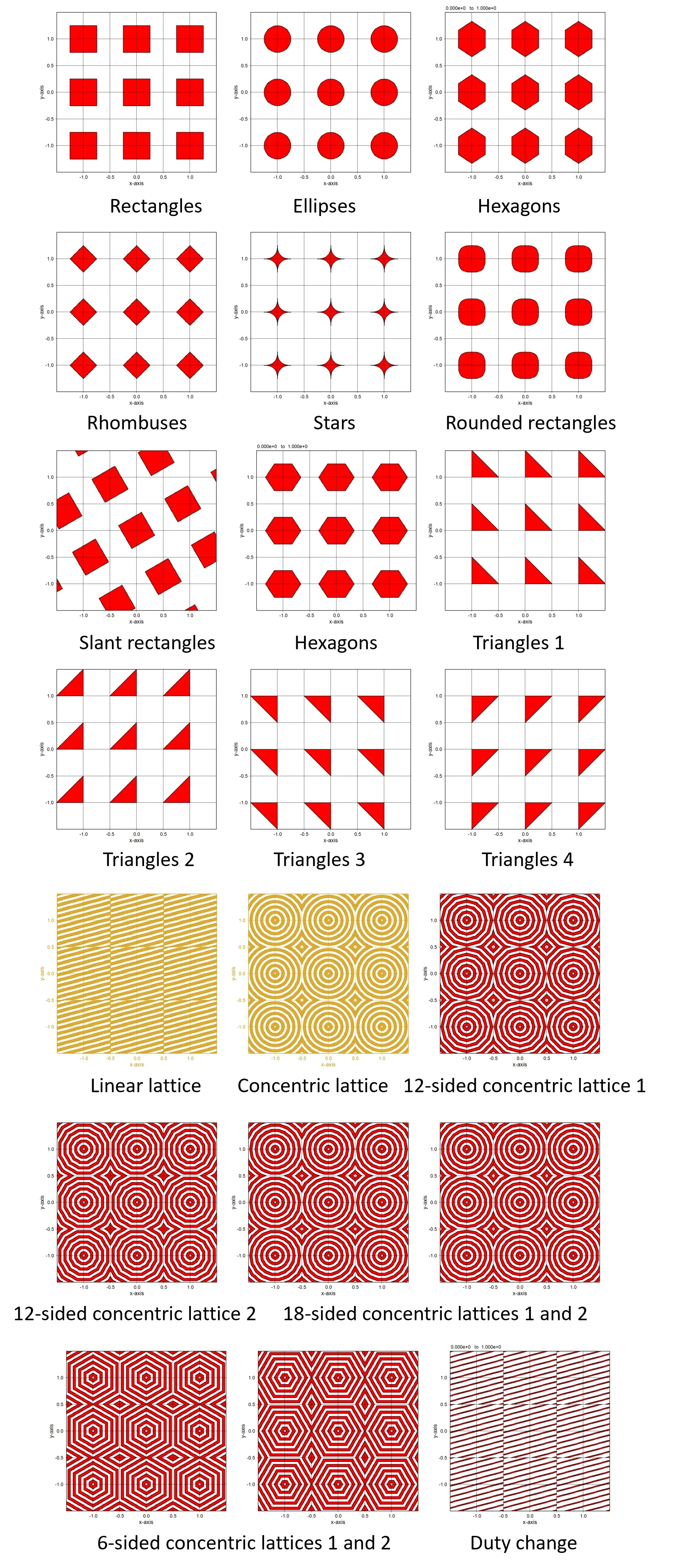
Of these, the following figures are defined by kt in the Internal box.
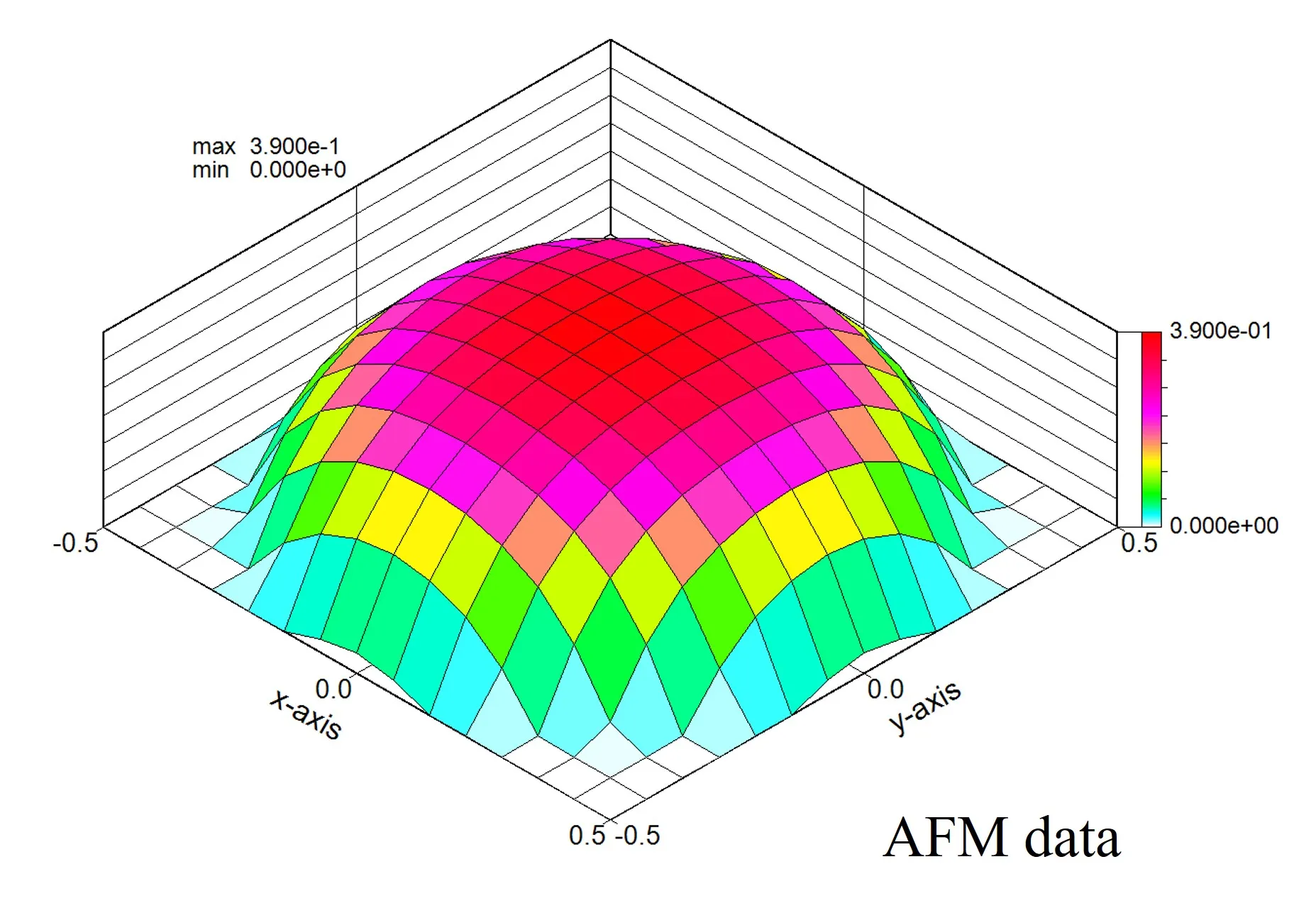
All shapes that cannot be defined internally can be defined using sub.dat. For example, a figure enclosed in four points (x1,y1), (x2,y2), (x3,y3), (x4,y4) described in sub.dat can be defined. As an expression of the measured value of the three-dimensional shape, there is height data at the evenly spaced mesh intersection points by using AFM (Atomic Force Microscope) shown below, but the cross-sectional figure of the data cut by the isometric plane (uniform height) is a collection of figures surrounded by four points, so it can be expressed by sub.dat.
Furthermore, by setting px and py, the periodic shape of these figures can be defined.
● How to set up sub.dat
This section describes how to convert four-point data compiled in excel into sub.dat and how to convert AFM data into sub.dat.
(1) Click the Clear button and select Wsf(FDTD).

(2) Set 2.0 for wdx and wdy, 0.02 for dxy and dz; register Si and -SiO2 in the Material setting field; click the ← button in the Base layer setting field to move to the edit panel.
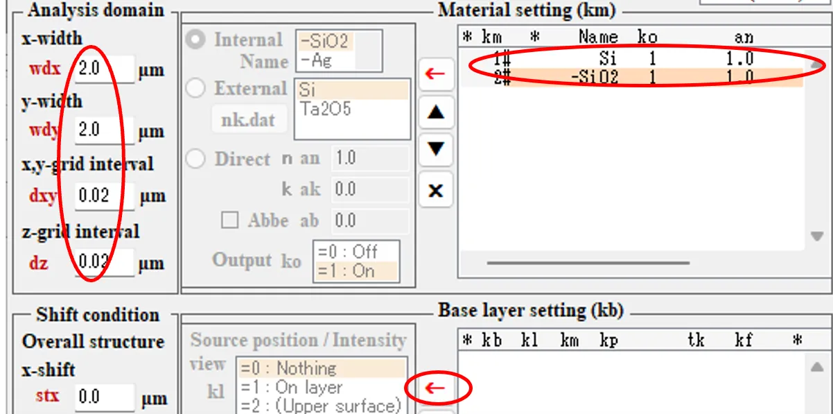
(3) Set tk to 0.02 (= height increment of AFM measurement) and click → button. Register the first base layer in the registration list.
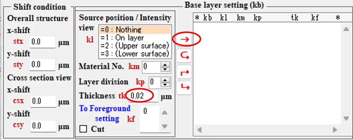
(4) Click on the ← button to go to the edit panel.
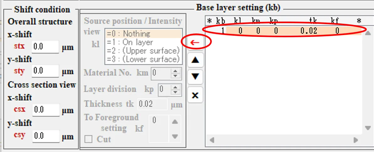
(5) Set tk to 0.02 and kf to 1 and click the ⮡ button. Register the second base layer in the list.
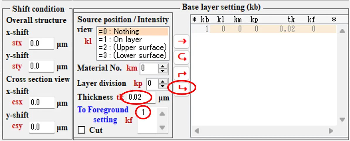
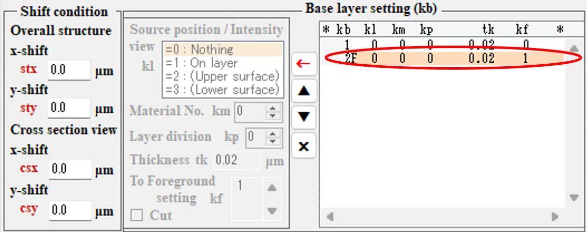
(6) When the Draw button is clicked, the background colour of the Draw button changes from pink to grey and the data in Wsems.dat is updated to the settings so far Wscnt starts drawing but closes.

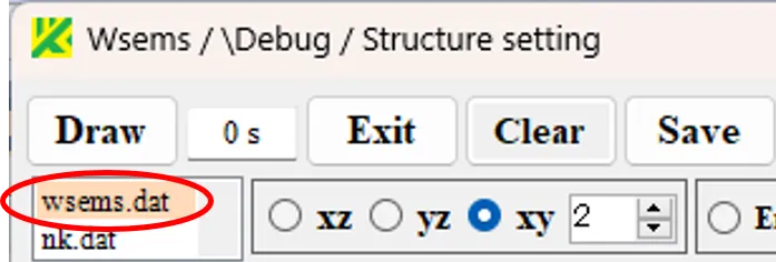
(7) Double-click wsems.dat in the result file box to display the information window (Info).
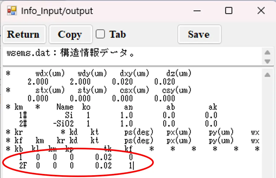
(8) Repeat copying and pasting layers 1 and 2 until you have a total of 22 layers.
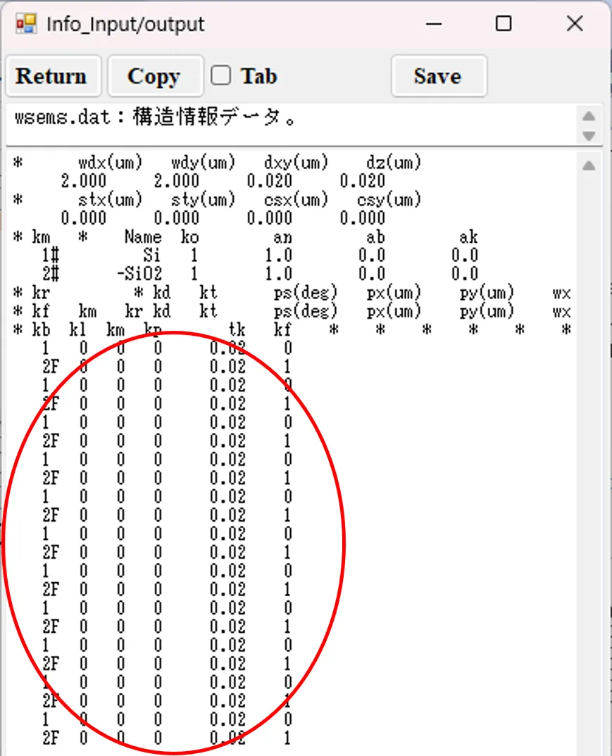
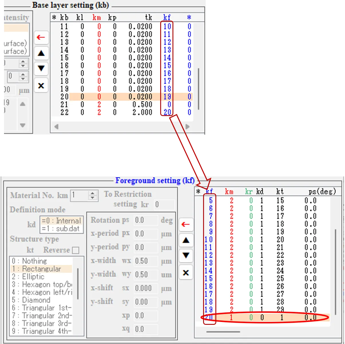
(9) Change kf to 2~19 with an increase of 1 from 2 for layers 3~20, 0 for layer 21 and 20 for layer 22; change tk to 0.5 for layer 21 and 2.0 for layer 22; change km to 2 for layers 21 and 22. However, be sure to use half-width input as full-width may cause malfunctions.
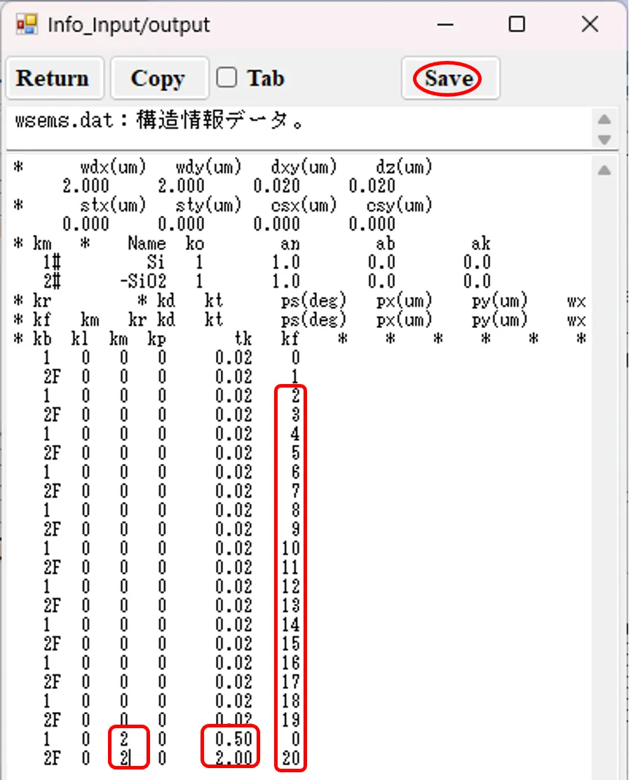
(10) When the Save button is clicked, serial numbers and horizontal misalignments are automatically corrected and registered in the Base layer setting field.
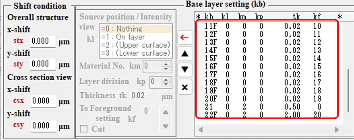
(11) Click the ← button in Foreground setting field to move to the edit panel. Set 2 for km, 1 (sub.dat) for kd, 1.0 for px,py.
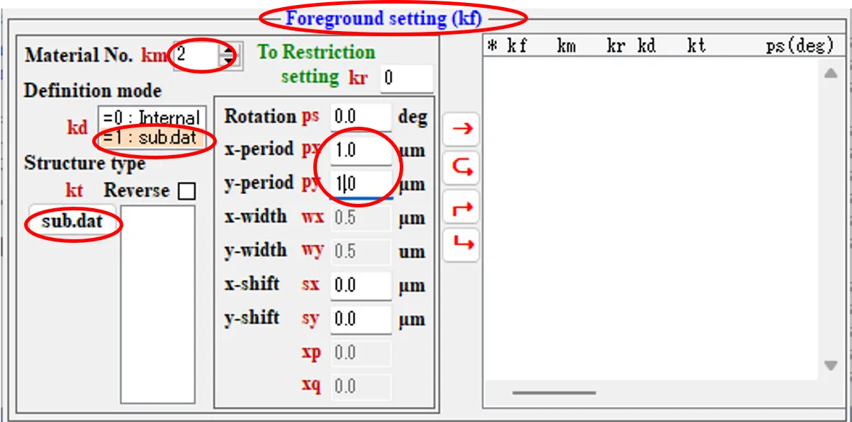
(12) Click on the sub.dat button to open the sub.dat setting window.

(13) Check the Points data button and paste the data from \samples\sub_data.xlsl in the left-hand box.
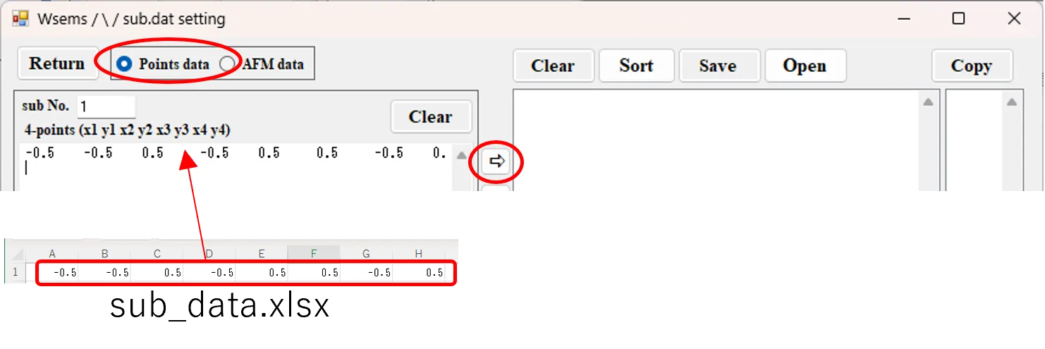
(14) Click on the button ⇒. Register the first data in the two lists on the right-hand side.

(15) Click on the top of the right-hand box list and select the data. To check, click on the Draw button and draw the cross-sectional shape.

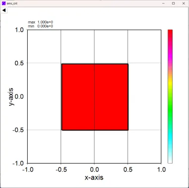
(16) Check the AFM data button and enter 11 in the sub No. box (or use the assigned value of 2). Paste the AFM data from sub_data.xlsl in the leftmost box. Note that the right boxes for dx and dy are the xy-directional intervals of the AFM measurement points and the right box for dz is the height-directional interval.
(Reference) In the box to the right of dz, the angle (theta) of the surface normal to the z-axis, the declination angle (phi) of the surface normal around the z-axis and the rotation angle (psi) of the measurement image around the surface normal can be added in units of deg, separated by spaces. If omitted, they are treated as 0.
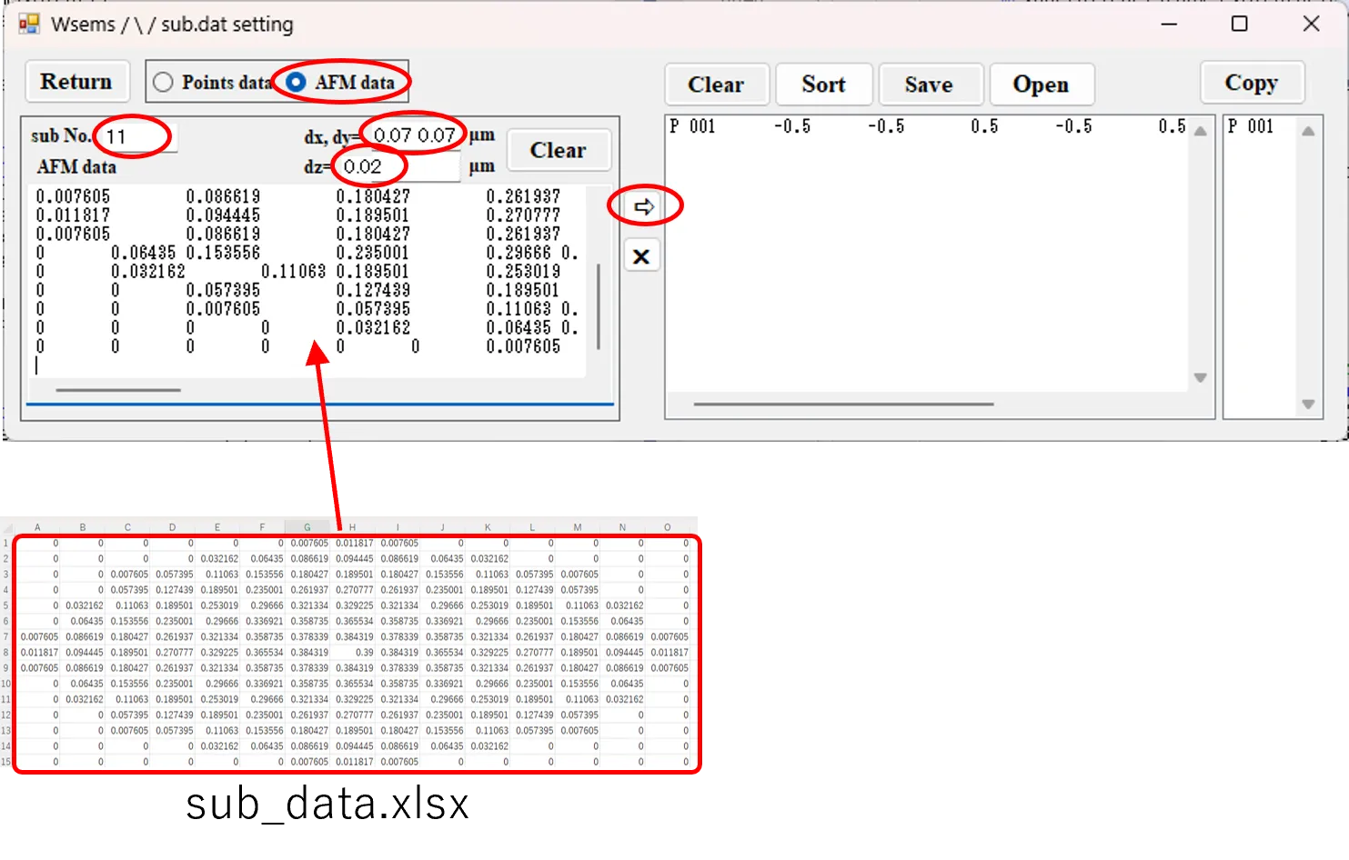
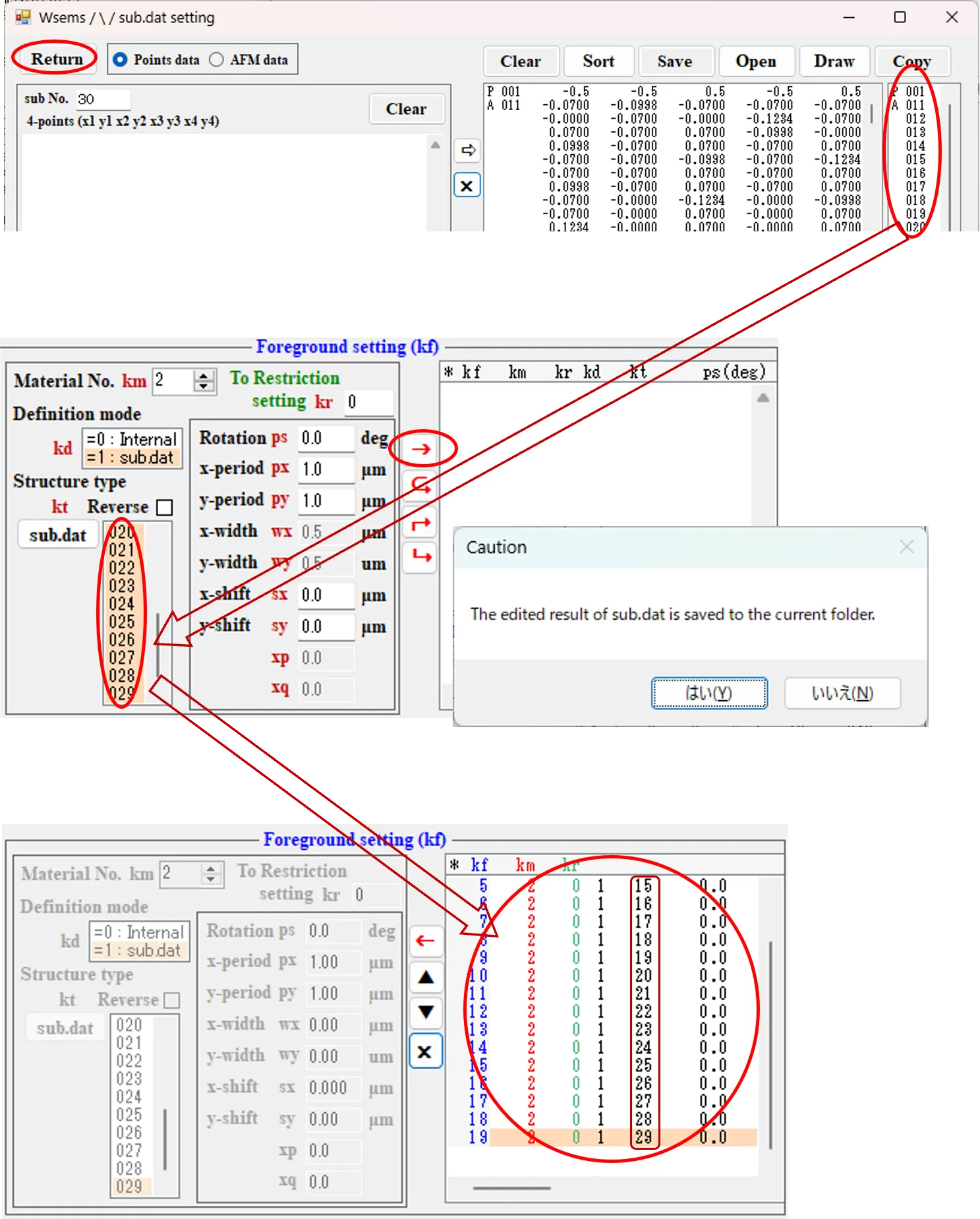
(17) Click on the button ⇒. Register the second data in the list with assignment numbers 11 to 29 (Sub No.).

(18) Select the data by clicking on the second line of the rightmost box list (A011, Sub No. 11); A 011 consists of several rows of 4-point data.

To check, click on the Draw button and draw the cross-sectional profile: a circular cross-section is represented by a collection of 4-point data. Similarly, you can view other cross-sectional profiles by selecting other lines in the right-hand box list.
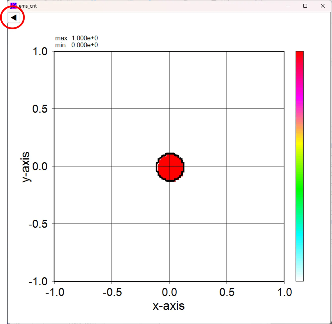
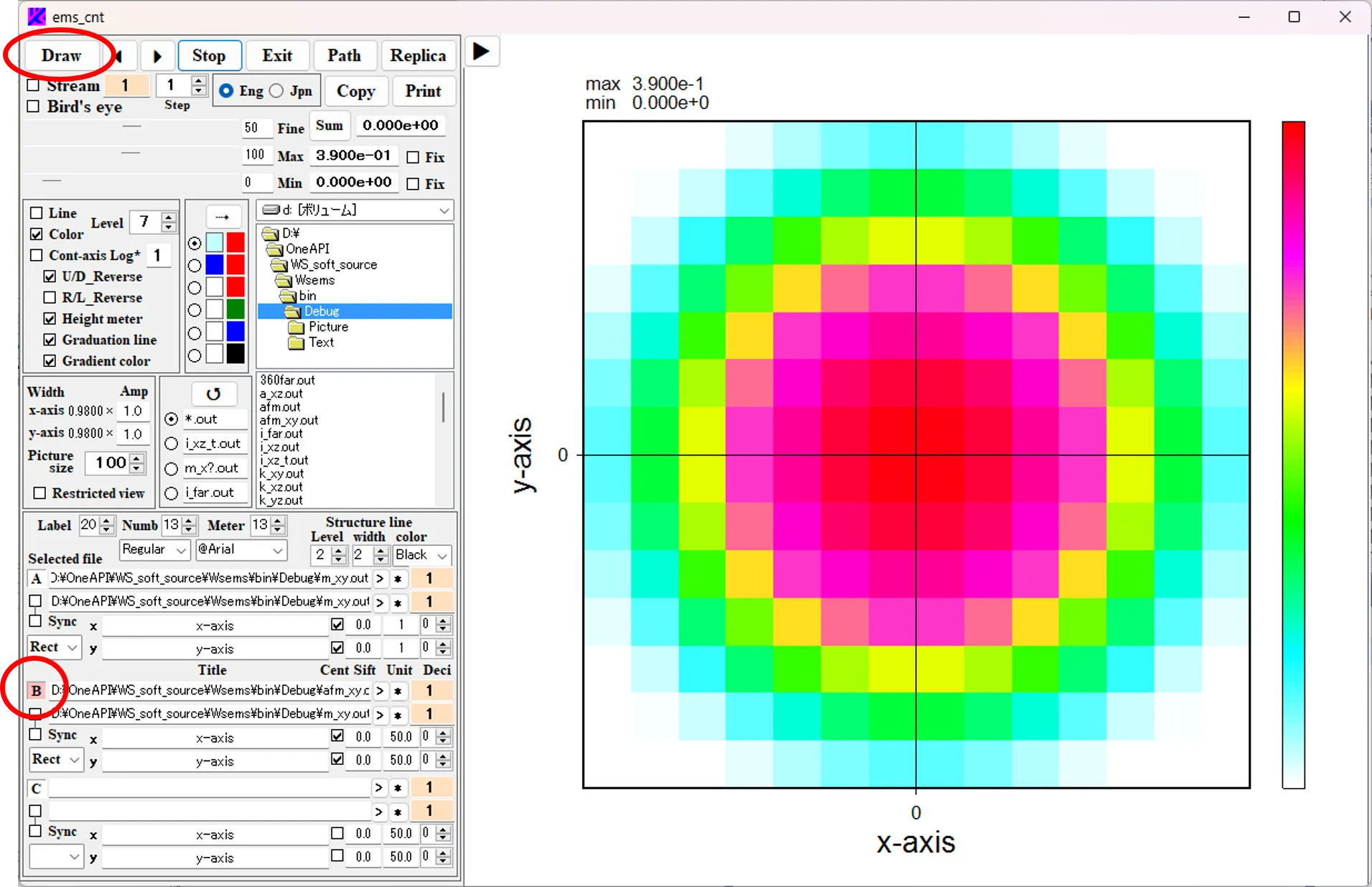
As a reference, click on the ◀ button in the diagram above to open the control panel, select the B button and click on the Draw button to draw a contour map of the AFM data (afm_xy.out).
(19) Side note: Check the Points data button, check the check box and enter 2 in the sub No. box. Paste the data from sub_data.xlsl in the far left box.
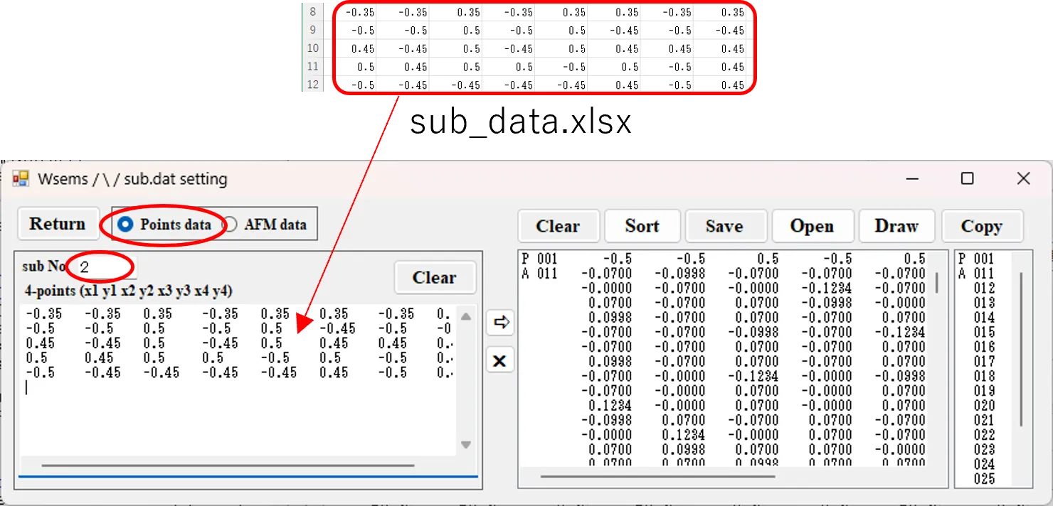
(20) Click the button ⇒; data from Sub No. 2 is added to the list.

(21) Clicking on the Sort button will sort the list in ascending order by sub.No.

(22) Click on P 002 in the right-hand box to select it. To check, click on the Draw button and draw the cross-sectional profile. If P 002 is not required, click the X button in the blue highlighted state to delete it.

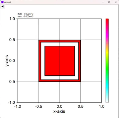
(23) Back to (18). Click on the Return button, answer ‘Yes’ to Causion and return to the Foreground setting field. The contents of the list in the right box are registered as serial numbers in sub.dat: drag 11-29 in the kt list to the right of the sub.dat button and click the → button with km=2 and px=py=1.0. Register foreground structures from kf=1~19 in the list. The kt number of the foreground structure recalls the serial number of the sub.dat.
(24) In the foreground structure of row 19 (kf=19), click on the ← button and go to the edit panel. Set km=1, kd=0 (Internal) and kt=1 (Rectangular), px=py=0.0, wx=wy=0.5.
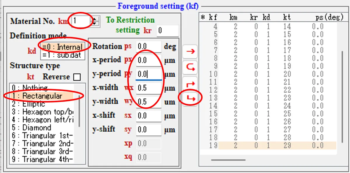
(25) Click the ⮡ button to register the 20th foreground structure in the list. The number of kf in the base layer calls up the foreground structure that is composed on top of it.
(26) Check xy button and set the right box to 20.

Click on the Draw button for confirmation, drawing the xy-section of the 20-layer structure. The structure is periodic because 1.0 was set for px and py in (11).
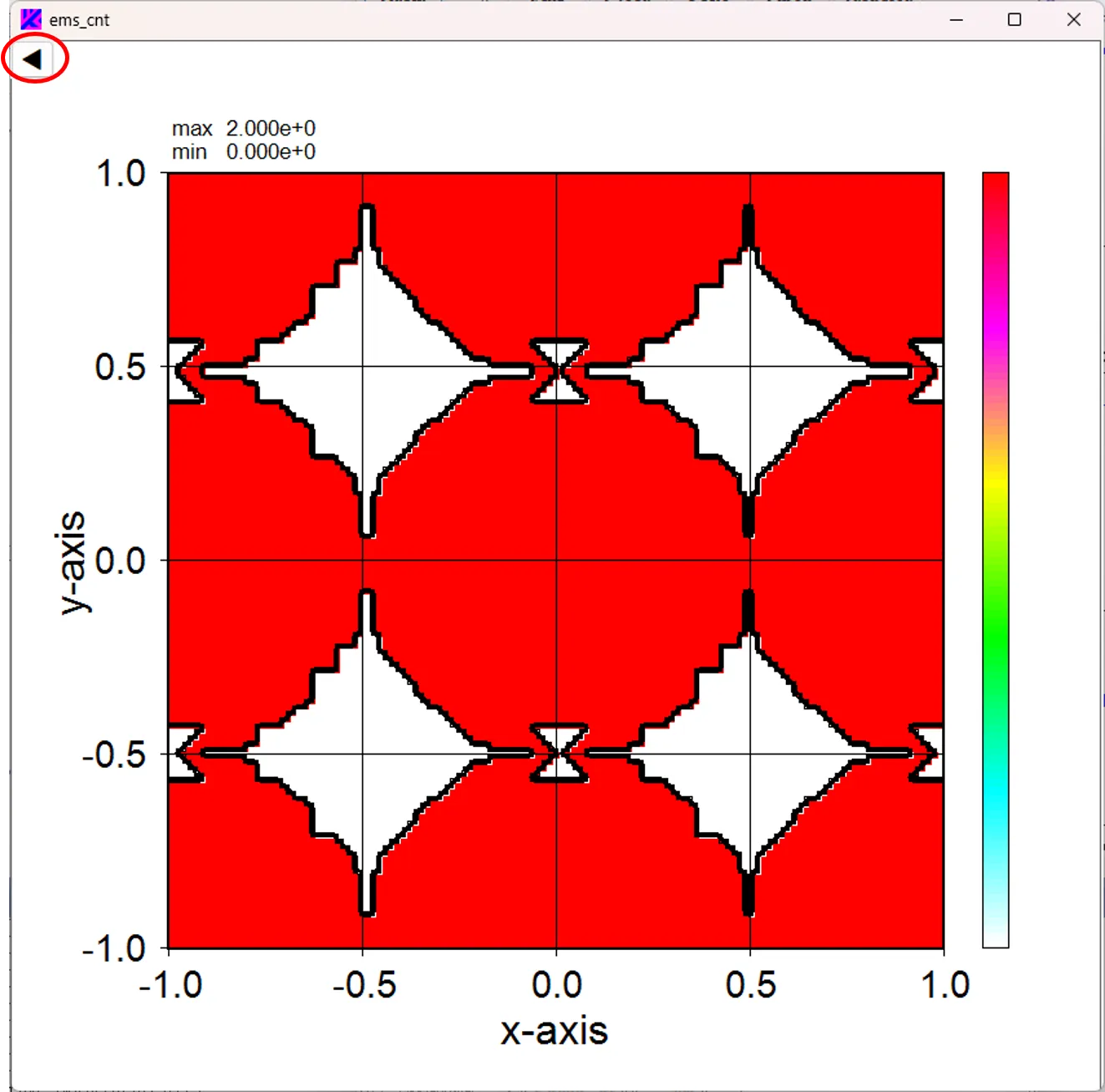
Click on the ◀ to display the Wscnt operation panel. Click on the ◀▶ buttons of the panel to check the cross sections of other layer numbers.
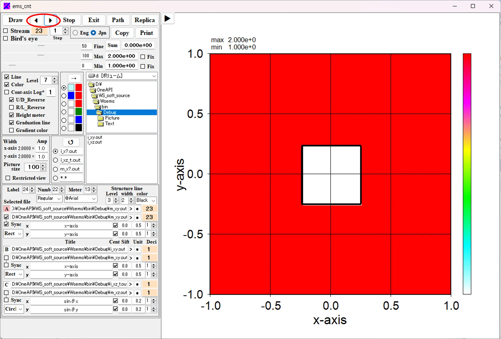
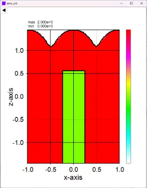
(27) Check xz the button.

Click on the Draw button to draw an xz-section of the structure.
Now we can represent the 3D shape by AFM measurements using sub_dat. Next, let's set the light source and perform the wave calculation.
(28) Click the Next button to open the Source setting window and set each parameter as follows.
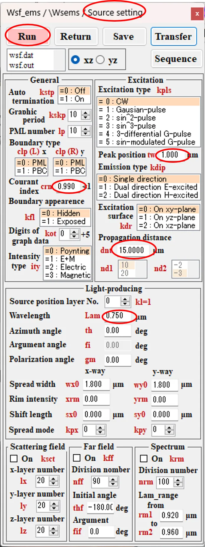
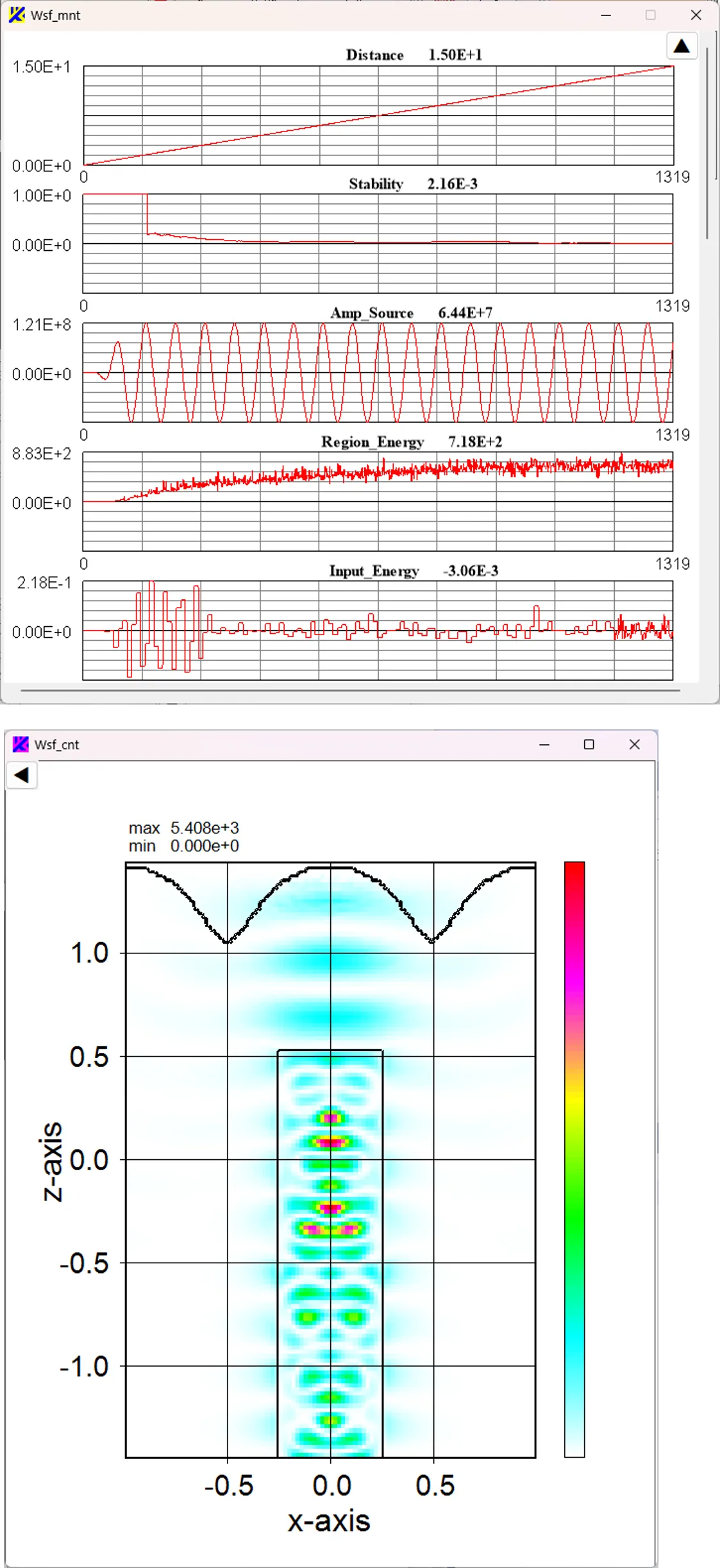
(29) When the Run button is clicked, the Dos window appears, the Wsf calculation is performed and at the same time the calculation status and the xz-section of the light intensity distribution are drawn by Wsmnt and Wscnt.
● Other ways of calling the sub_dat setting window
There are other ways to invoke the sub_dat setting window besides methods (11) and (12).
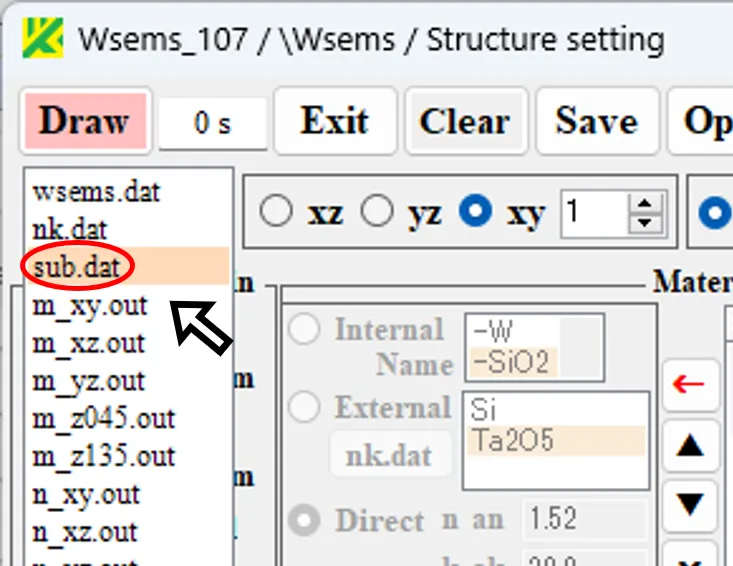
(30) Move the mouse pointer over the result file box on the Source setting window and double-click 'sub.dat' in the box to open the information window.
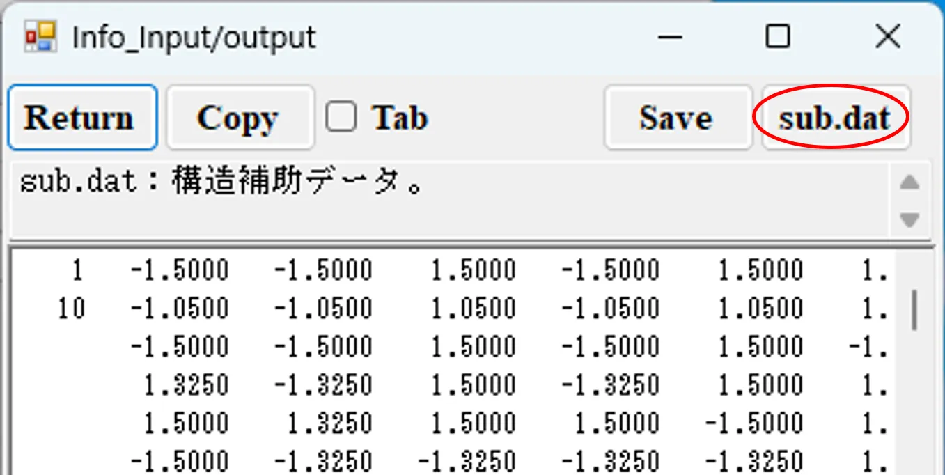
(31) Click on the sub.dat button on the information window and the sub.dat setting window as same as in (12) appears.
● Preparation for serial calculation (for single conditions).
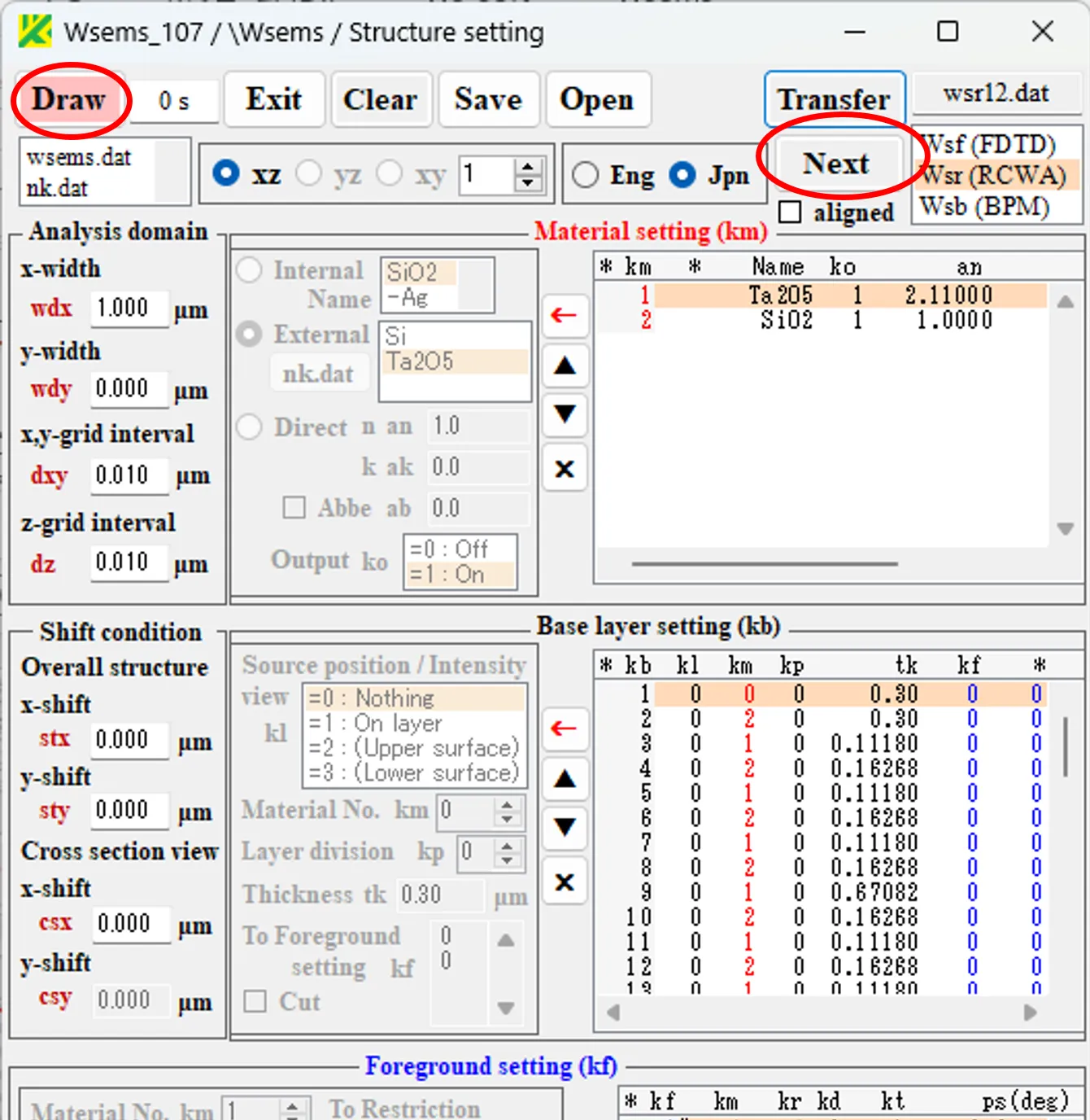
(1) Click on the Clear button and select Wsr (RCWA); click on the Transfer button.

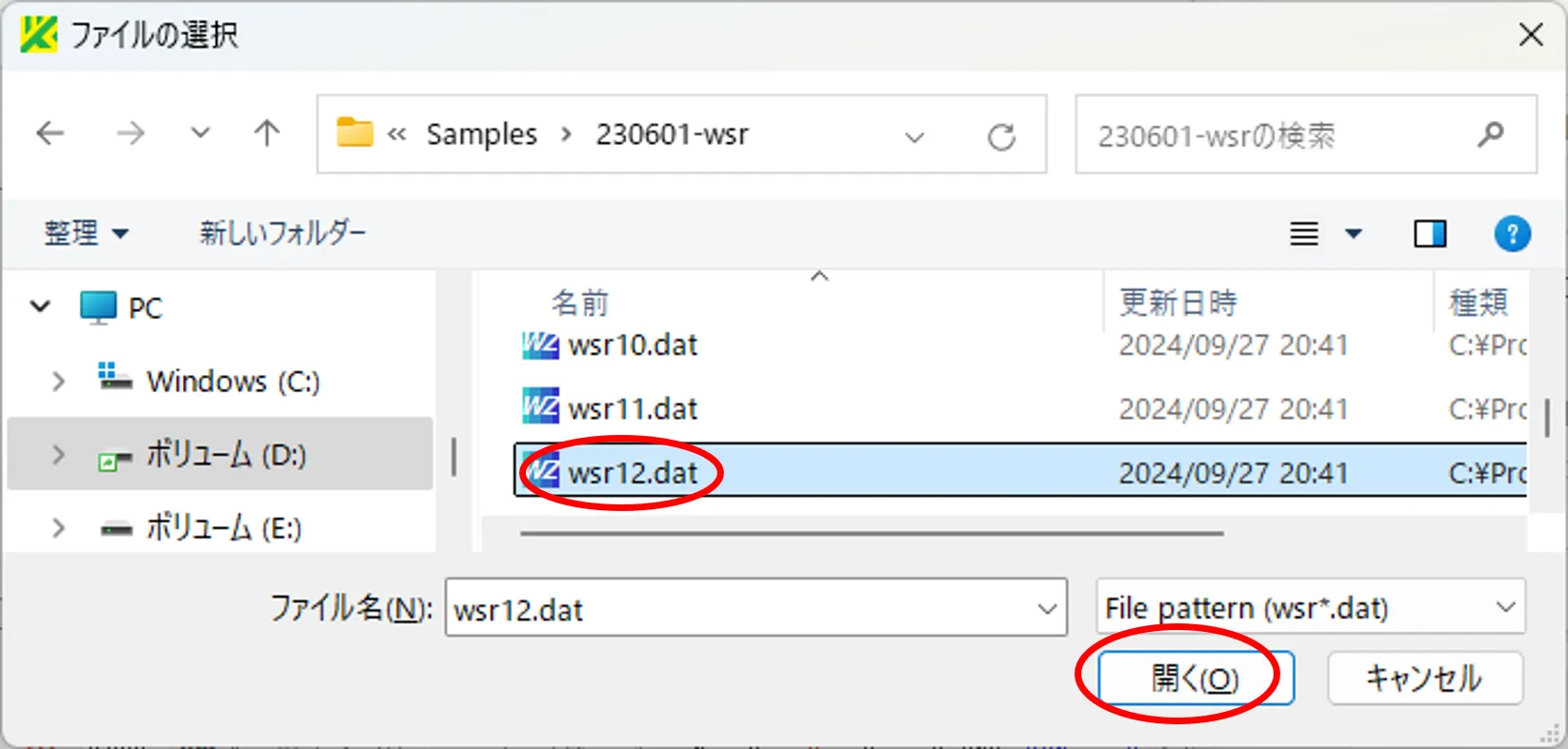
(2) In the file selection window, select the file (wsr12.dat) from the \Samples\230601-wsr directory and click the Open button. The structure information is extracted from the file contents and reflected in the Structure setting window.
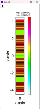
(3) Clicking on the Draw button opens the Wscnt window and the xz-sectional structure is drawn.
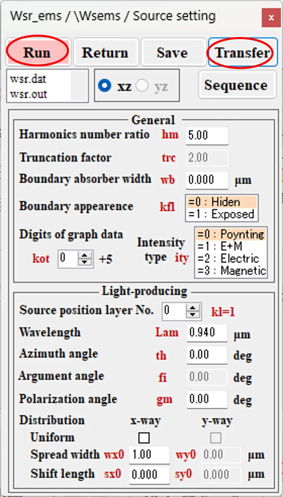
(4) Click the Next button to open the Source setting window, click the Transfer button, select a file (wsr12.dat) from the directory \Samples\230601-wsr in the file selection window and click the Open button. The light source information is extracted from the file content and reflected in the Source setting window.
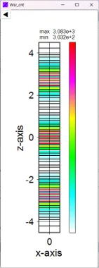
(5) When the Run button is clicked, the Dos window appears and the calculation of Wsr is performed. When the calculation is finished, the Dos window disappears and the calculation results are drawn by Wscnt.
● Serial calculation with Wsbch
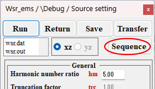
(6) Click on the Sequence button to open the Sequential window.
(7) Check the Wavelength button on the Sequential window and set each parameter as follows.
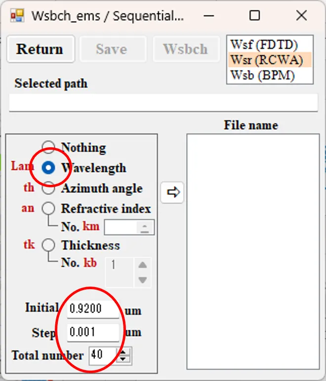
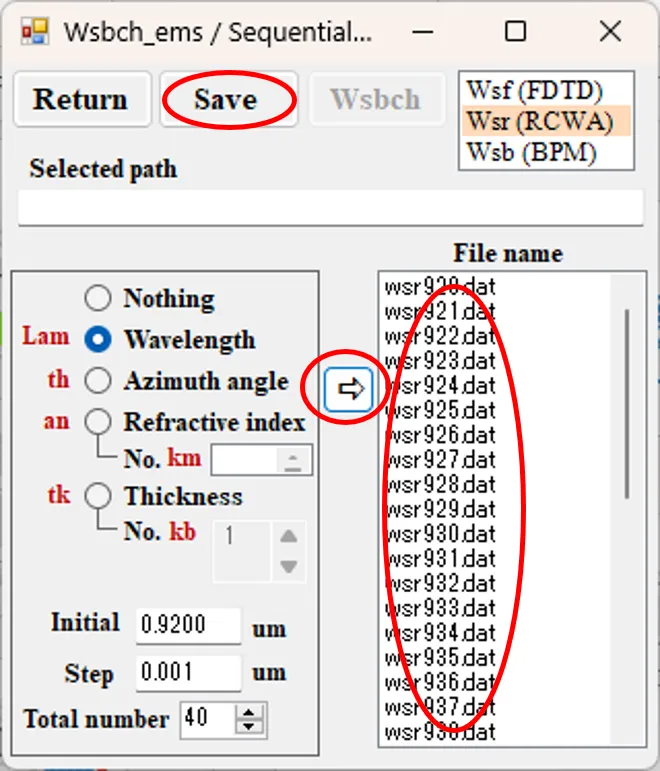
(8) Click on the ⇒ button to register the names in the File name box. 40 names are generated in 0.001 increments, starting from wavelength 0.920. The names corresponding to the parameter are automatically assigned.
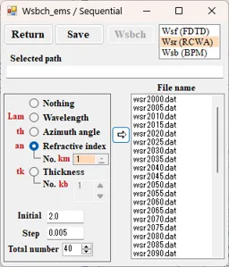
(9) For reference, if the Refractive index button is checked and the respective parameters are set, file names are generated with the refractive index of material number km as a parameter.
If the Thickness button is checked and each parameter is set, file names are generated with the layer thickness of the specified layer number kb as a parameter.
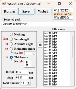
(10) Back to (8), click the Save button, select a folder in the selection window and click the OK button. To create a new folder, enter a folder name and press Enter key to confirm the entry.
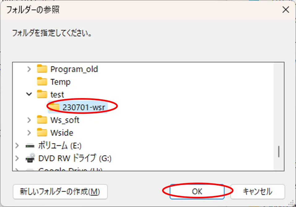
(11) The selected folder is listed in the Selected path box and a file with the names listed in the File name box are generated in that folder.
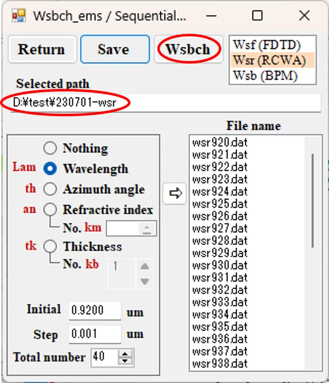
(12) Clicking on the Wsbch button opens Wsbch, where the data for the serial calculation are set with the names corresponding to the parameters.
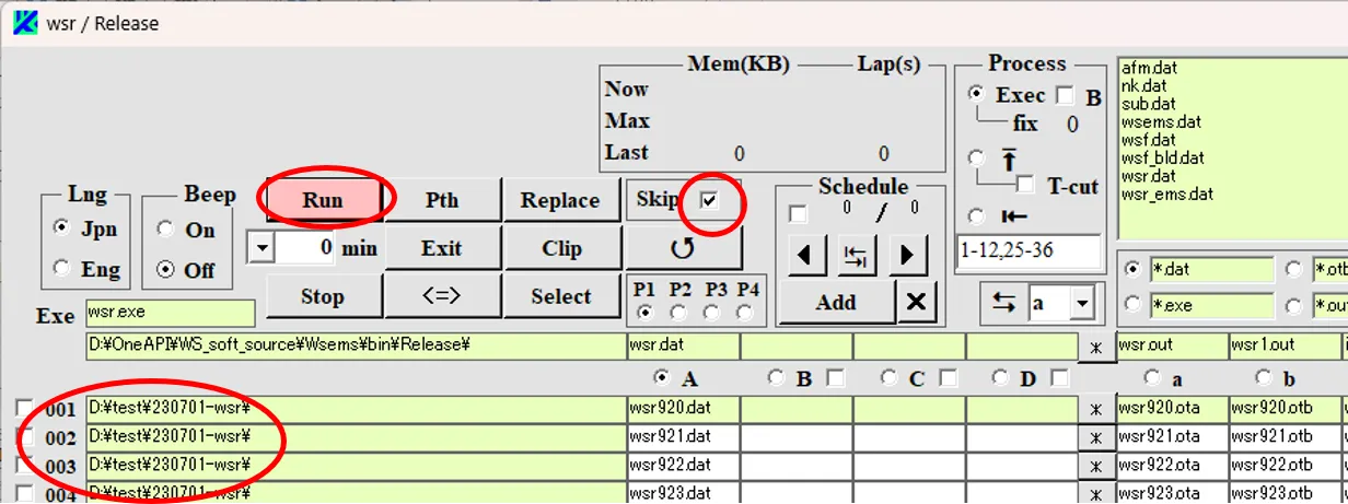
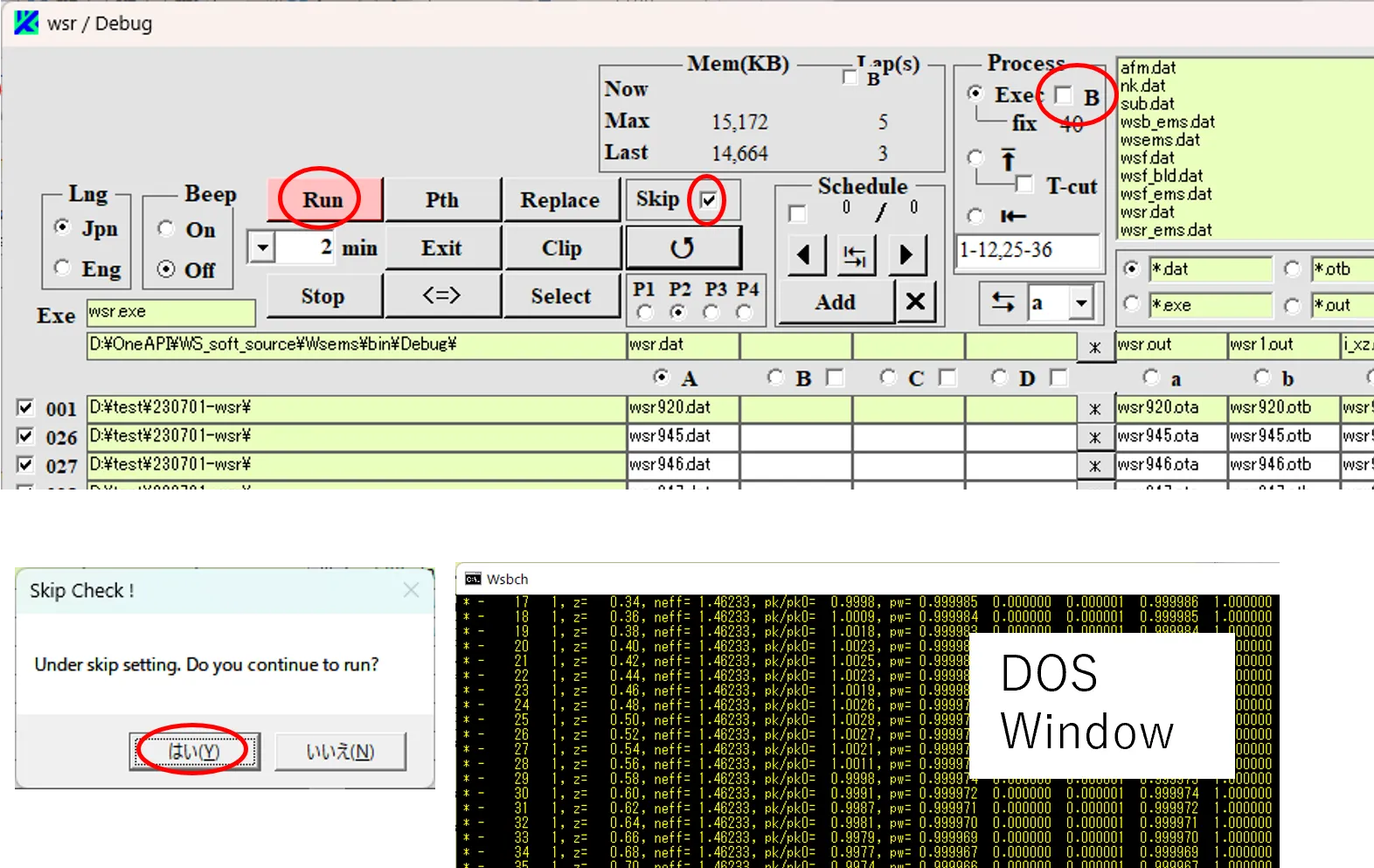
(13) When the Run button is clicked, a confirmation window appears, and when ‘Yes’is clicked, the Dos and Wscnt windows appear and serial calculation begins. If the calculation has already been performed, it will be skipped. If recalculation is required, uncheck the Skip box before clicking the Run button. Dos and Wscnt windows can be hidden by checking the box B in the Process box, which reduces the busy state associated with displaying the windows.
The calculation flow is as follows. Input file ① (e.g. wsr920.dat) in the storage folder is copied to input file ② (wsr.dat) in the execution folder. The output file ④ (wsr.out etc.) generated by the execution file ③ (wsr.exe) in the execution folder is copied to the output file ⑤ (wsr920.ota etc.) in the storage folder. When the calculation is finished, the DOS windown disappears and the next stage of calculation starts. The calculation proceeds to the button P2 and the data for the end of the calculation is checked in the leftmost box ⑥ in sequence.
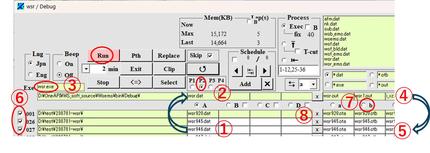
Check the box b ⑦ and click on the * button ⑧ to open the Edit window, where you can check the contents of the output result wsr920.otb for the wavelength of 920 nm.
● Summarising the calculation results
(14) The output results of continuous calculations with wavelength as a parameter are stored in wsr920.otb to wsr959.otb. We want to concatenate these results into one consolidated result.
After the calculation is finished, check the ⭱ box. Right-click on the path box ① to change the directory ② to the same folder as the path box. Set the file pattern to *.otb to display the *.otb file in the file list ③.

(15) Click button P1 to return to page 1 and click on the box in the first row of column A to make that row disappear.
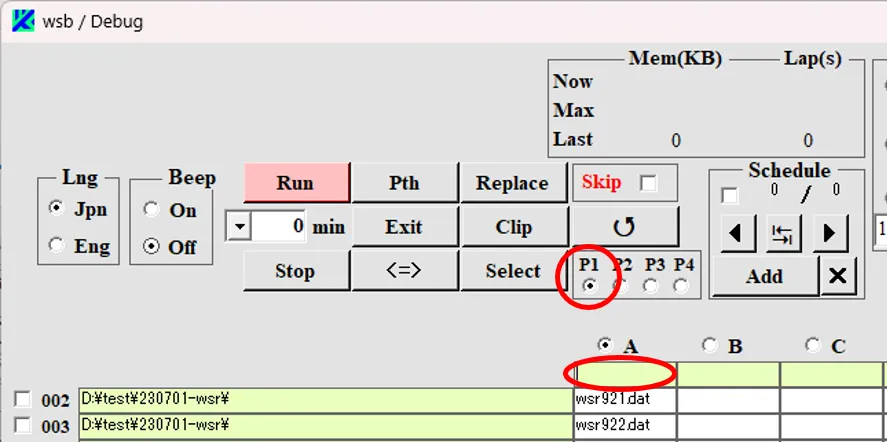
(16) If the consolidation is the first time and the file list ③ does not contain any files of *c.otb, pressing the Enter key registers only the files of *.otb in column A in order.
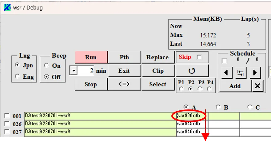
If a file with *c.otb is included in the file list ③ due to a previous consolidation, pressing the Enter key will also register the file with *c.otb in column A. Click on the box containing the *c.otb file to clear the display.
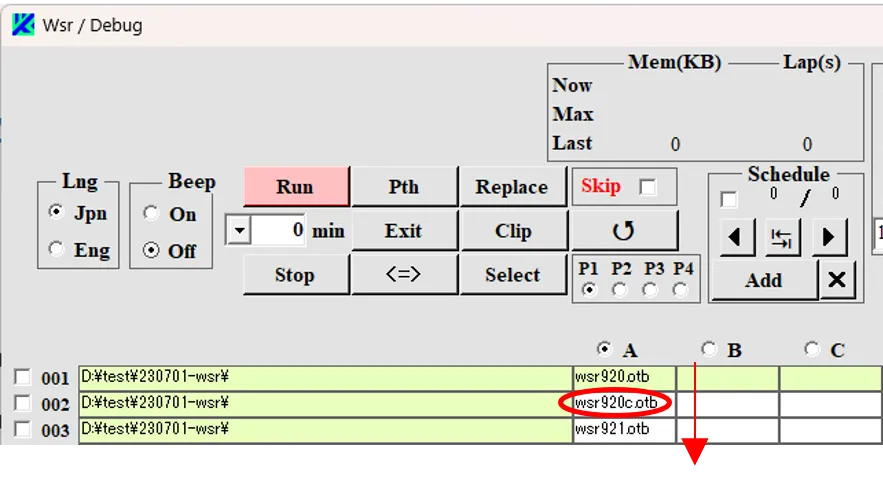
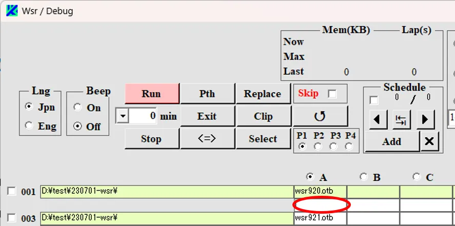
(17) When the Run button is clicked, the *.otb files in column A are concatenated in sequence and the concatenated results are stored in the box that appears above the top with the file name *c.otb.
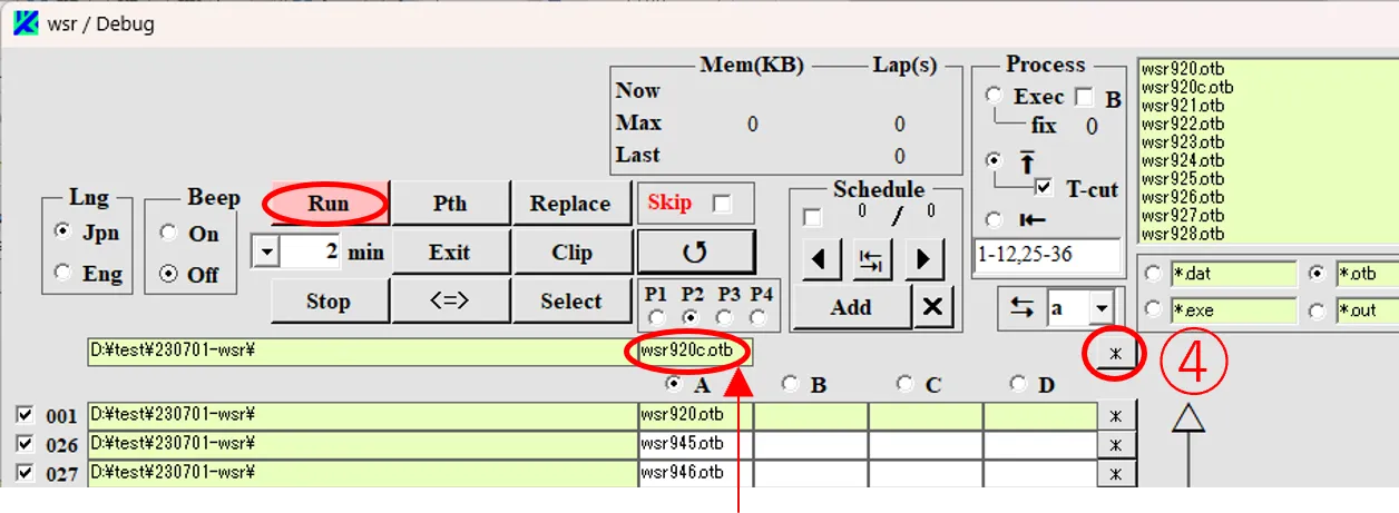
Clicking the * button (4) to the right of the line in the storage box (the *c.otb file box) opens the Edit window, where the results of the merging can be viewed. The first line (the line containing Transmitted) for the second and subsequent files has been deleted because the consolidation was executed with the ⭱ box checked.
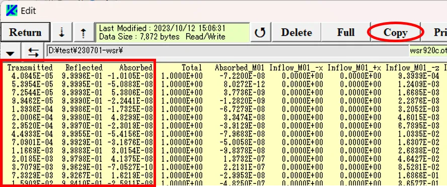
(18) By clicking on the Copy button and pasting the content into Excel, graphing of the results for serial calculations can be achieved.
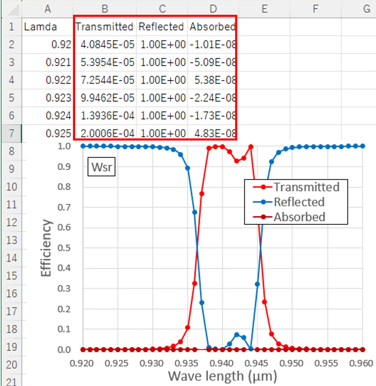
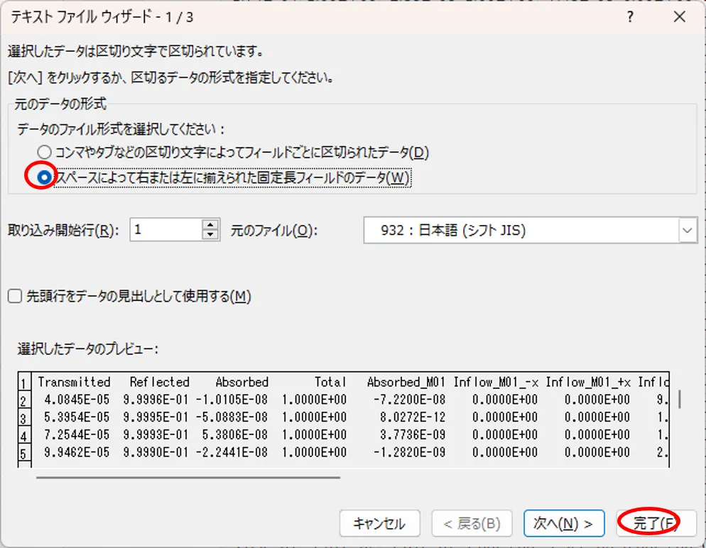
However, the pasting should be completed by checking the fixed value fields in the Excel text file wizard.
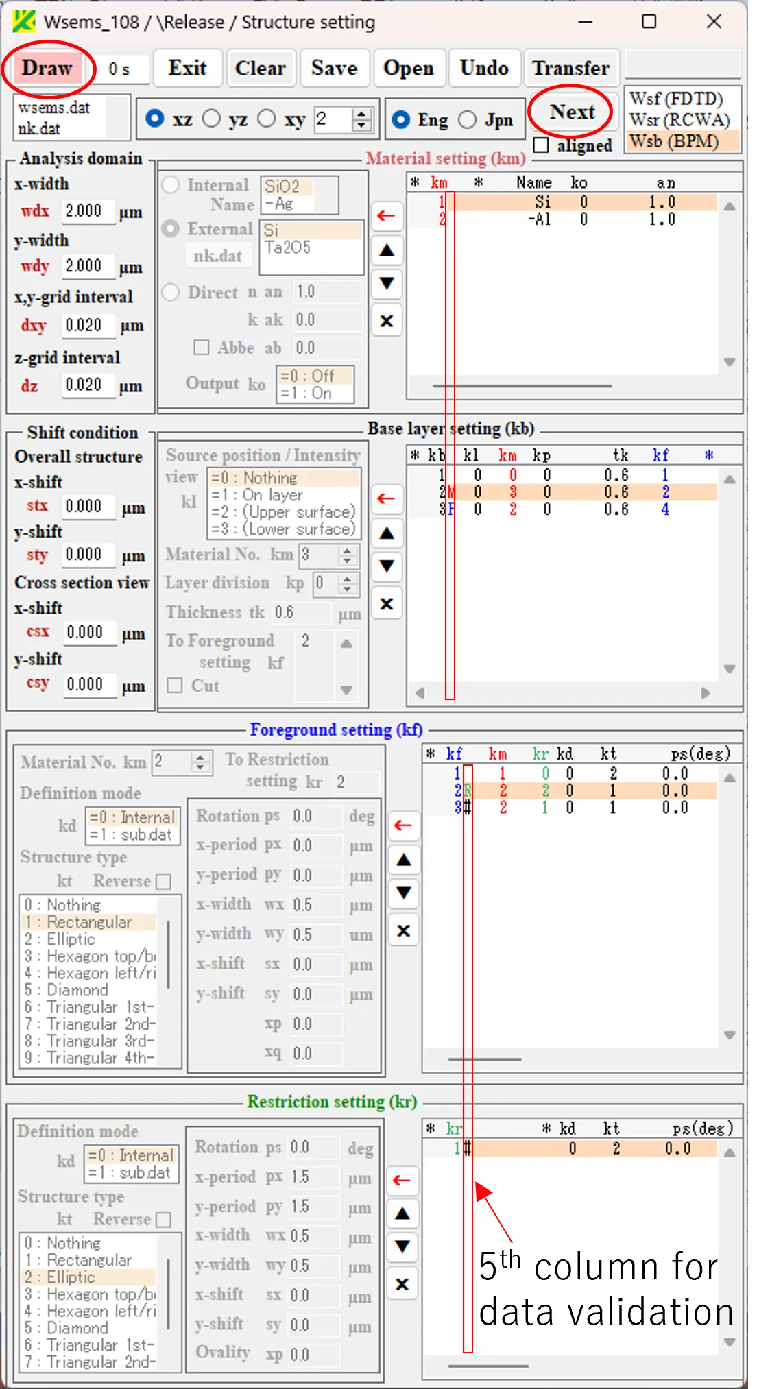
(1) The following example, in which the "M", "F", "F" and "#" entries remain, illustrates how to check and correct incorrect entries.
(2) The following message appears when the Draw or Next button is clicked.
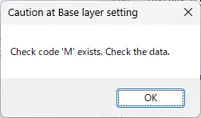
(3) Click OK button and modify the data so that the "M" disappears.

(4) The following message appears when the Draw or Next button is clicked.
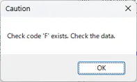
(5) Click OK button and modify the data so that the "F" disappears.

(6) The following message appears when the Draw or Next button is clicked.
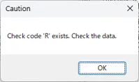
(7) Click OK button and modify the data so that the "R" disappears.

(8) Click on the Draw button to draw the cross-sectional view. The input data is normal because the Caution window does not appear because all the "M", "F" and "R entries have been removed. Note that the "#" is not a mistake, only that it is not referenced.
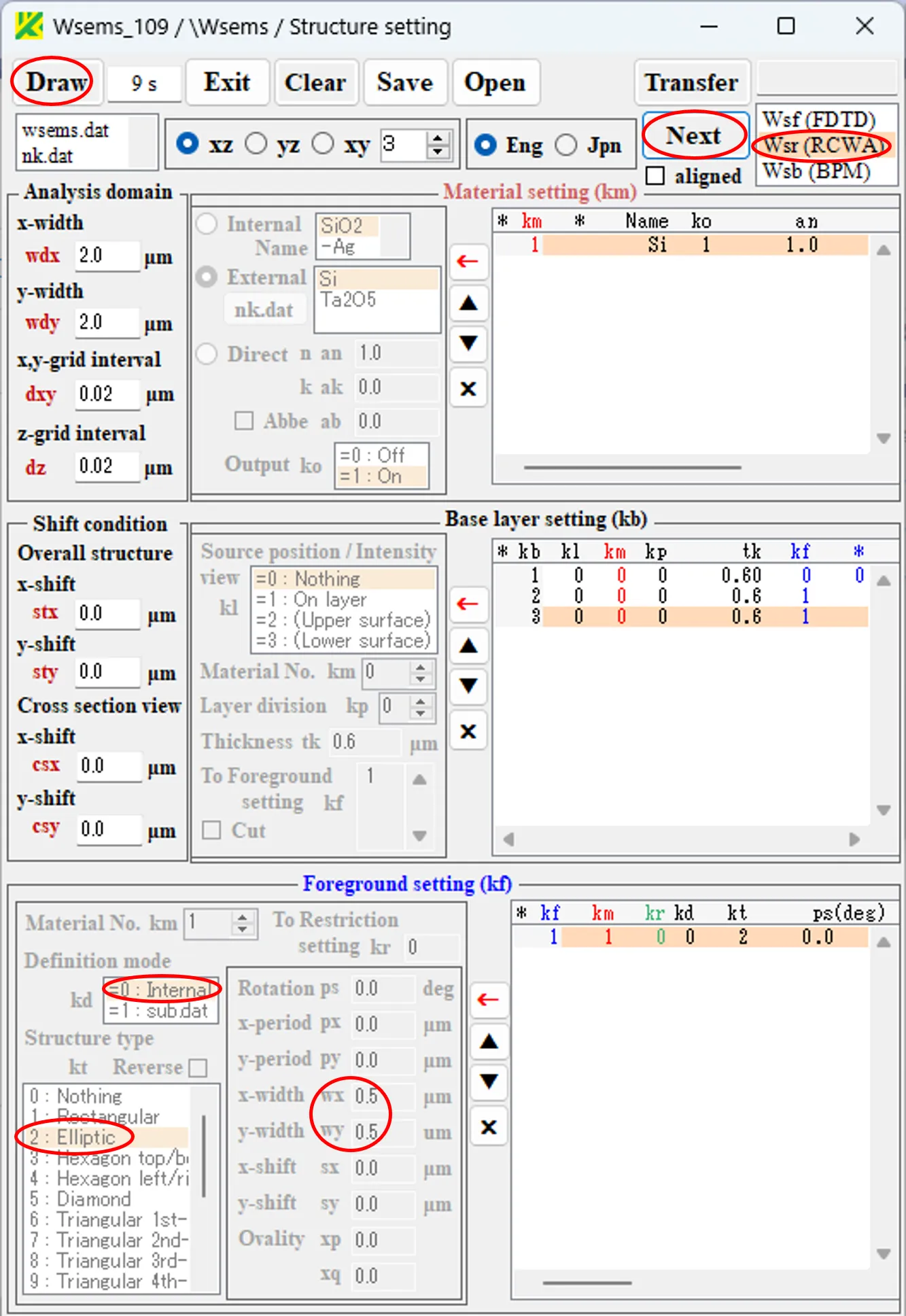
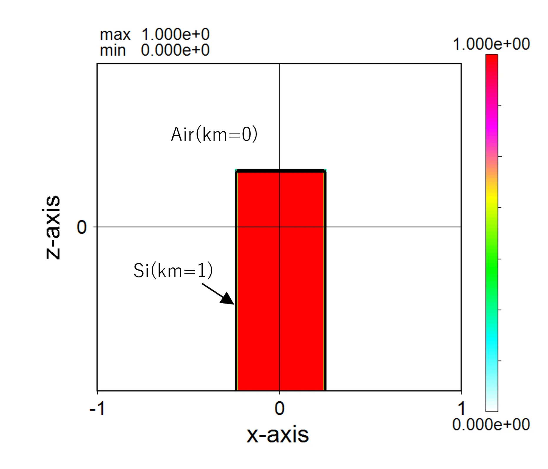
(1) Select Wsr (RCWA) and set the Structure setting window as shown below. The first line of the Foreground setting field is kd=0 (Internal), kt=2 (Elliptic), and wx=wy=0.5.
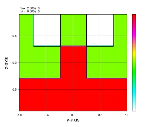
(2) Click on the Draw button to draw a cross-section of the structure. The cross-section is a columnar structure of Si with a diameter of 0.5 µm in air.
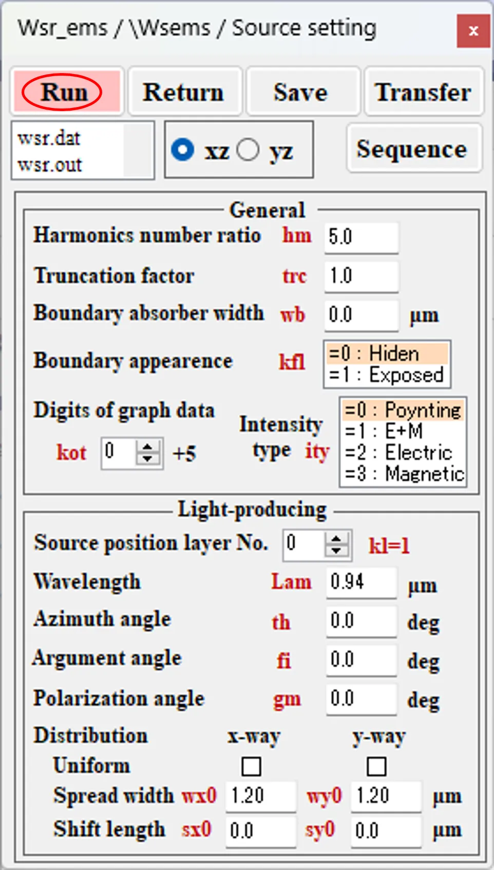
(3) Click the Next button and the Source Setting window appears. Set the parameters as shown in the diagram below and click the Run button to execute the wave calculation.
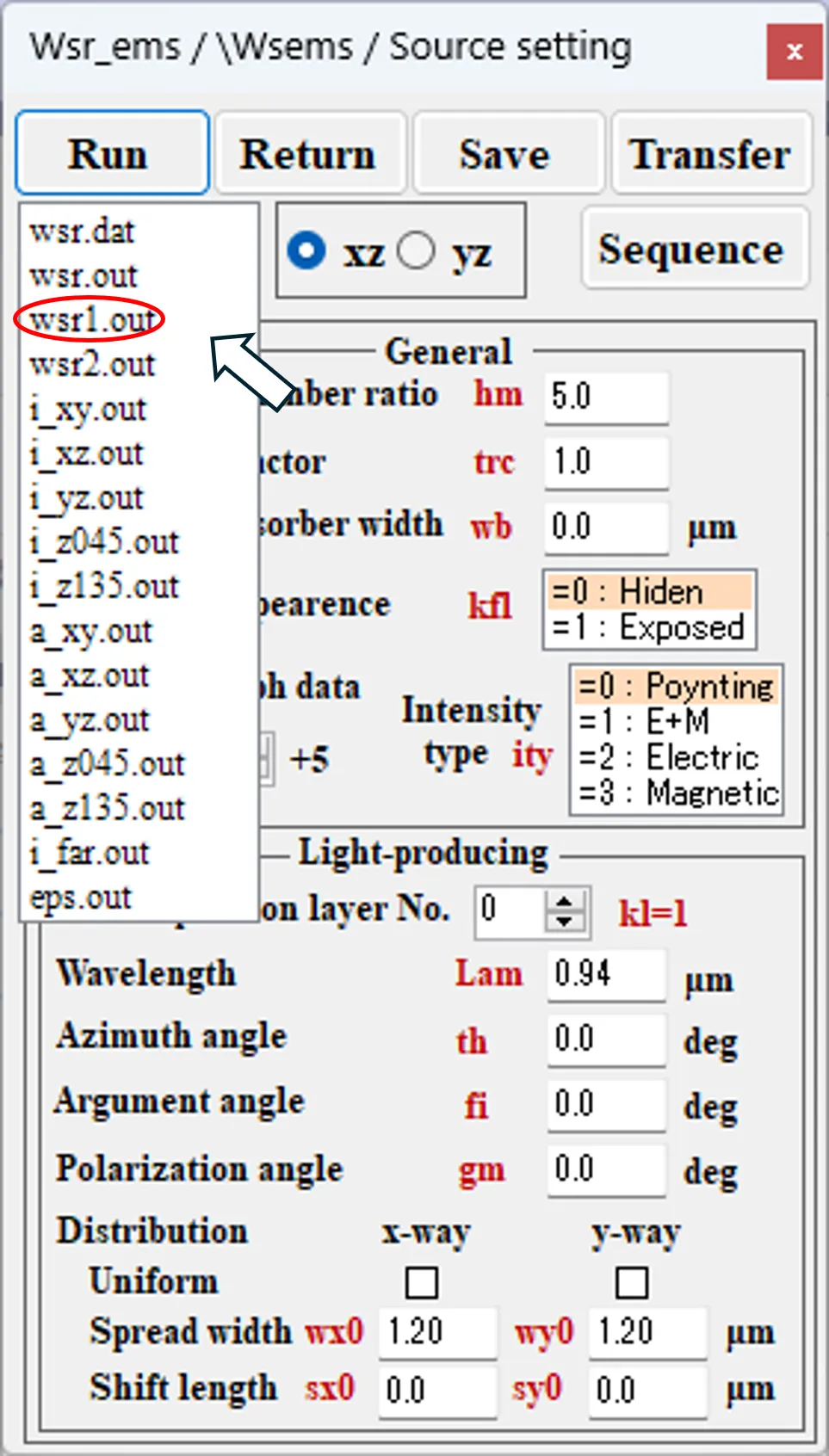
(4) When the calculation is finished, the background of the Run button changes from grey to pink: select wsr1.out from the result file box below the Run button, double-click it and the information window appears.
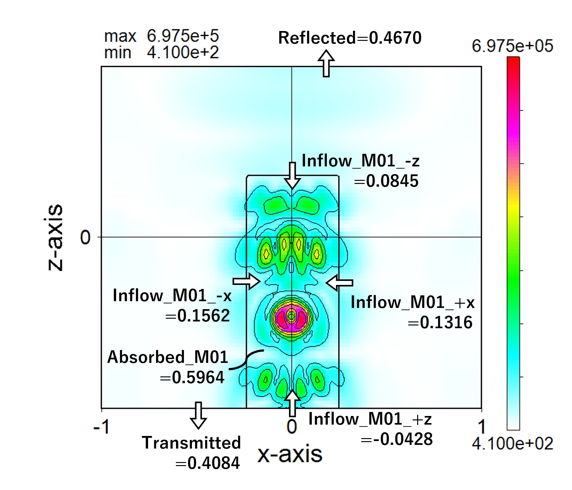
(5) The range ① labelled M01 on the information window is the result of the light amount calculation for material 1 (Si with km=1), and from left to right is the absorbed light amount and the inflow into the six cross sections (-x, +x, -y, +y, -z and +z axis cross sections in that order). However, the inflow into the cross-sections is the vertical component of the inflow, while the negative inflow means the outflow.

(6) The figure below shows the light intensity cross section (i_xz.out) that appears at the end of the calculation in (4) above, with the inflow at each cross section indicated by arrows corresponding to the contents of the Information window. Note that the figure is drawn with the z-axis inverted, so the axis polarity is reversed.
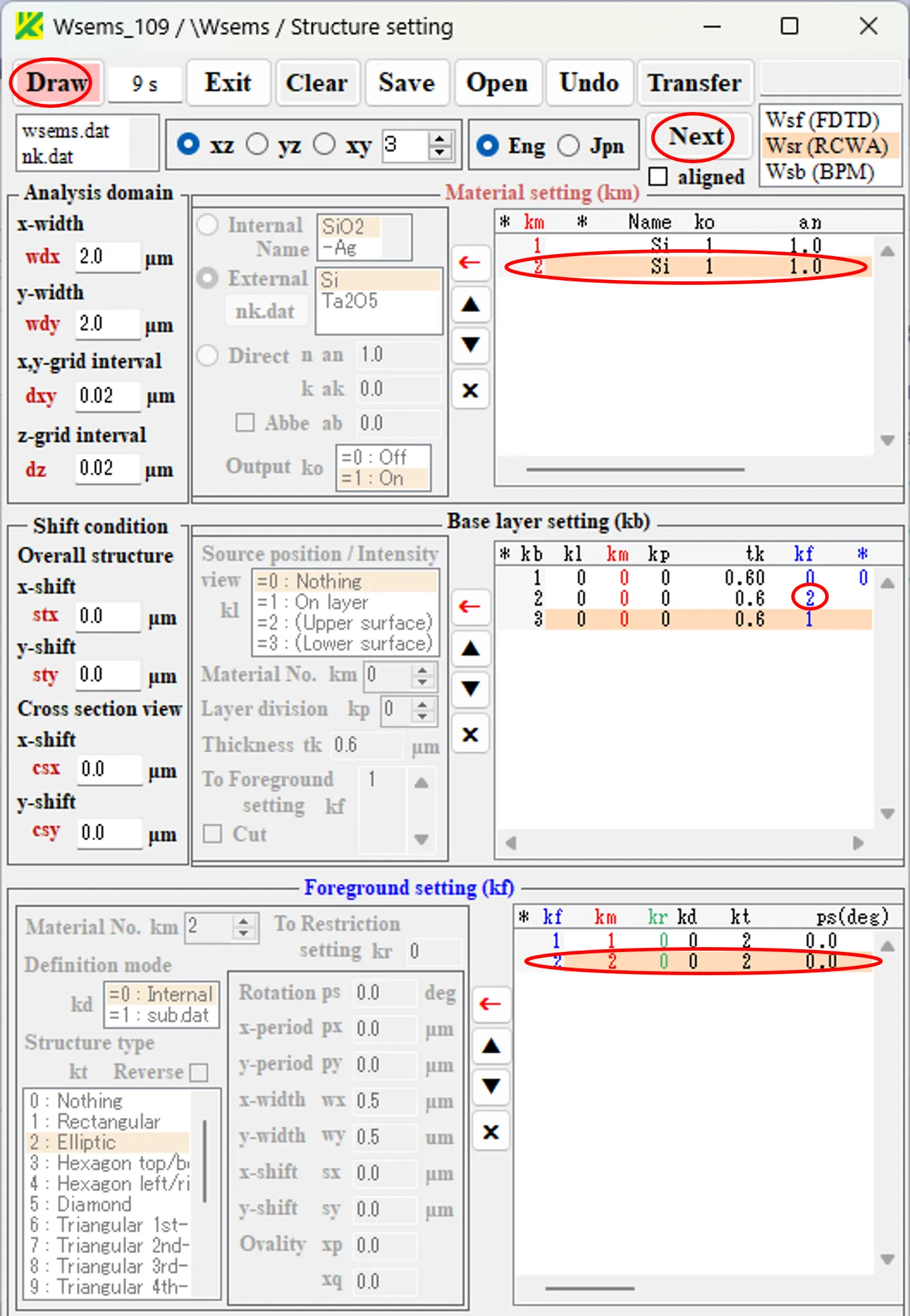
(7) Next, to calculate the light amounts in the upper half of the columnar structure, the Structure setting window is changed as shown below. That is, add Si to the second line (km=2) in the Material setting field, change kf=2 for the second layer (kb=2) in the Base layer setting field, and add a second line (kf=2) in the Foreground setting field under the same conditions as the first line and change km=2.
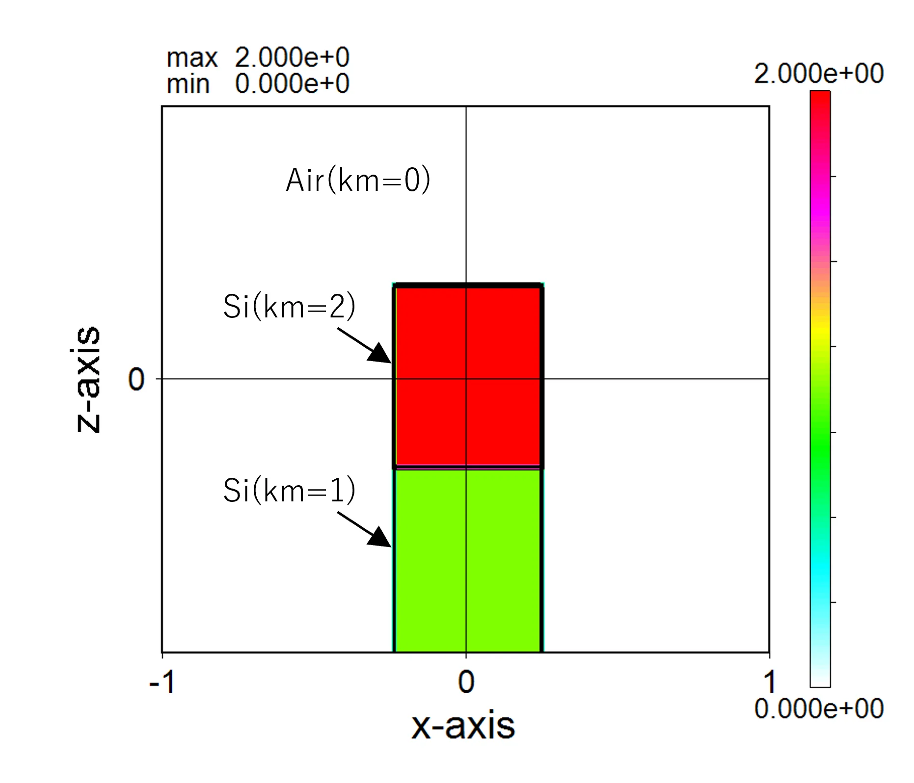
(8) Click on the Draw button to draw a cross-sectional view of the structure. A columnar structure of Si with a diameter of 0.5 µm is equally divided into upper and lower sections.
(9) Click on the Next button to bring up the Source setting window, then click on the Run button to execute the wave calculation.

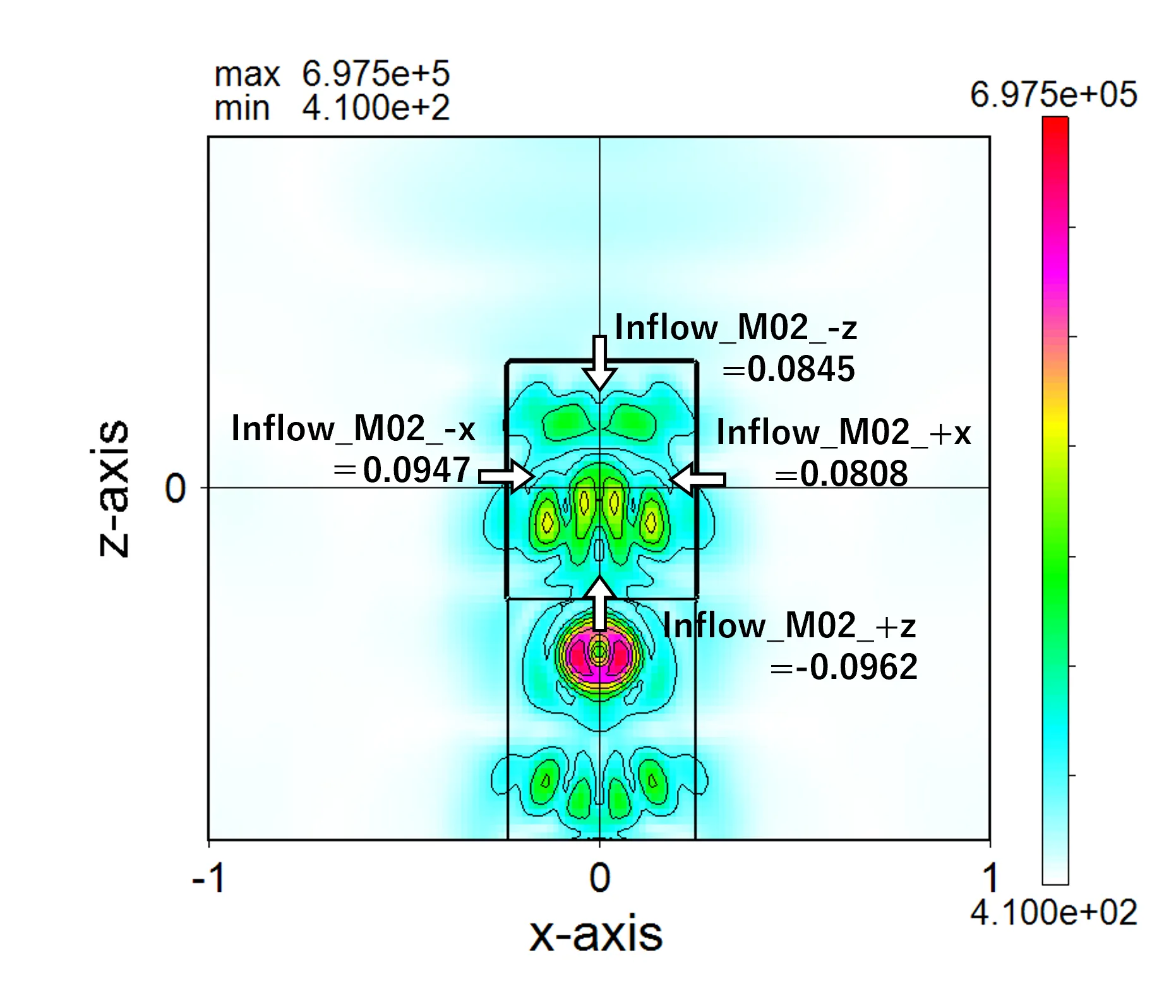
(10) Select wsr1.out from the results file box below the Run button and double-click it, and an information window will appear: on the information window, the range ① labelled M01 is the calculation results for material 1 (km=1, lower half of Si) and the range ② labelled M02 is the calculation results for material 2 (km=2, upper half of Si) and are, respectively, from left to right, the amount of absorbed light and the amounts of inflow into the six cross sections (-x, +x, -y, +y, -z, +z axial cross sections in that order).

(11) The figure below shows the light intensity cross section (i_xz.out) that appears at the end of the calculation in (9) above, with arrows indicating the inflow at each cross section of material 2, corresponding to the contents of the Information window.
Thus, to measure the amount of inflow and absorbed light in an arbitrary space, a unique material number can be assigned corresponding to the space, and the calculation results are output to wsr1.out using that material number. Output results of wsr1.out in Wsr correspond to wsf1.out in Wsf and wsb1.out in Wsb, respectively.
● 2. Usage examples using sample data
● 3. Sample calculation examples
● 4. Viewing information about parameters and buttons
● 5. Basic operation of the structure settings panel
● 6. Structure definition
● 7. Output files in the definition structure
● 8. Wave calculation
● 9. Limitation
Learn more
● 10. Material Data Settings (nk.dat)
● 11. Structural Auxiliary Data Settings (sub.dat)
● 12. Serial Caluculation (Wsbch)
● 13. Identification and correction of incorrect input
● 14. Light amount detection
1. How to install Ws_soft ▲top
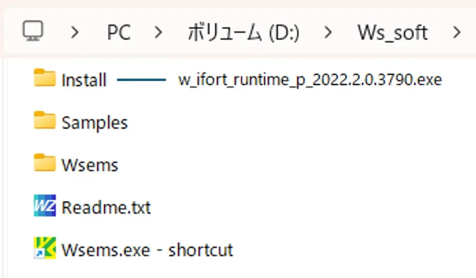
(1) Unzip the downloaded zip file and the folder Ws_soft will be extracted. Copy this folder under the drive (e.g. C or D drive) to install the software.(2) Remove the folder of Ws_soft from the drive to uninstall the software.

2. Usage examples using sample data ▲top
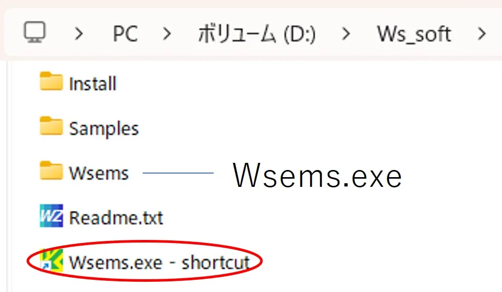
(1) Click Wsems.exe-shortcut in the Ws_soft folder.
(2) If the protection window appears, click on 'More info', and then click the run button that appears in the lower left corner.

(3) After the Structure setting window of Wsems appears, select Wsf (FDTD) in it and click the Transfer button.

(4) On the file selection window, select a file (wsf08.dat) from the '\Samples\230601-wsf' directory and click the Open button.

(5) The Structure setting window is updated and click the Draw button.

(6) The Wscnt window appears and the cross-sectional shape is displayed.

(7) On the Structure setting window, click the Next button.

(8) The Source setting window appears, and click the Transfer button in it.

(9) On the file selection window, select a file (wsf08.dat) from the '\Samples\230601-wsf' directory and click the Open button.

(10) The Source setting window is updated and click the Run button.

(11) The Wsmnt window and the Wscnt window appear, and the calculation progress and cross-sectional intensity distribution are displayed in real time.


(12) Move the mouse pointer over the result file box on the Source setting window.

(13) The result file box expands downward.

(14) Double-click on one of the files (i_xz_t.out) in the result file box to bring up an information window.


(15) When you click the Draw button, Wscnt is automatically launched and the calculation result is redrawn.

(16) Go back to (12) and double-click one of the files (mnt.out) in the result file box to display the information window.

(17) When you click the Draw button, Wsmnt is automatically launched and the calculation result is redrawn.

3. Sample calculation examples ▲top
Try other sample data in the same way as above. Calculation times are also given.● Calculation examples for sample data in folders of \Samples are shown below.
(1) Calculation examples for sample data in \Samples\230601-wsf

(2) Calculation examples for sample data in \Samples\230601-wsr

(3) Calculation examples for sample data in \Samples\230601-wsb

● Calculation examples for sample data in folders of \Samples\Comparison are shown below.
(4) Calculation examples for sample data in \Samples\Comparison\230601-wsf. Paid for only wsf_9.dat (Limitation).

(5) Calculation examples for sample data in \Samples\Comparison\230601-wsr. Paid for only wsr_9.dat (Limitation).

(6) Calculation examples for sample data in \Samples\Comparison\230601-wsb. Paid for only wsb_9.dat (Limitation).

4. Viewing information about parameters and buttons ▲top
(1) Double-click the parameter box.
(2) The parameter definition information window (Info) appears, and the corresponding parameter is displayed in red. All parameters in the boxes in the Enable state are double-clicked to display the definition information on the Information window.

(3) When you hover the mouse pointer over a button in the Enable state, the operating information is displayed in the tooltip.

5. Basic operation of the structure settings panel ▲top
Let's explain the basic operation of the structure setting panel.When you click the ← button, the contents of the registration list are moved to the edit panel, and you can edit them.

Clicking on one of the four red buttons completes the edit, and the result of the edit is reflected in the registration list.

Let's take the definition of the material as an example and explain it concretely.
(1) After clicking the Clear button to initialize the panel, click the ← button in the Material setting field.

(2) Select SiO2 in the Internal box. Click the → button to register the first line.

(3) Click the ← button in the Base setting field.

(4) Select -Al in the Internal box. Click the ↳ button to register the second line.

(5) Move the specified item in the registration list up with the ▲ button.

(6) Move the specified item in the registration list down with the ▼ button.

(7) Delete the specified item in the registration list with the × button.

(8) When you click the ← button, the focus shifts to the left and you can edit it.


(9) When you perform an edit operation (-Al selection) on the left side, the → button appears.

(10) If you click the ⮎ button in (9), the focus will return to the right without reflecting the editing result.

(11) If you click the ↱ button in (9), the editing result will be inserted above.

(12) If you click the → button in (9), the editing result will be overwritten.

(13) If you click the ↳ button in (9), the editing result will be inserted on the lower side.

6. Structure definition ▲top
The following three-dimensional structure is defined in three steps.
● First, in the procedure (1) - (6) below, the background layers of kb = 1 - 27 composed of air (km = 0) are sequentially defined with tk as the film thickness.
(1) After initializing by clicking the Clear button, uncheck the aligned button and click the ← button in the Material setting field.

(2) Select 'SiO2' from Internal box. Click the → button to register the first line. Click the ← button in the Base layer setting field.


(3) Film thickness tk = 0.5. Click the → button to register the first line. Click the ← button.


(4) Film thickness tk=0.02, kf=1. Click the ↳ button to register the second line.


(5) Repeat (3) - (4) while increasing the value of kf by 1 until kf = 25.

(6) Film thickness tk=2.0, kf=0. Click the ↳ button to register the last row.


● Next, according to the procedure (7) - (11) below, assign the foreground structure defined in lines 1 - 25 of the Foreground setting field to the background layer for which the value of 1 - 25 is set for kf above.
(7) Click the ← button in the Foreground setting field.

(8) km=1, kd=0, kt=2, px=py=0.0, wx=wy=0.244, sx=sy=0.0. Click the → button to register the first line. It is a foreground structure corresponding to kf = 1 (the background layer for kb = 2).


(9) Click the ← button and set wx,wy=0.420. Click the ↳ button to register the second row. It is a foreground structure corresponding to kf = 2 (the background layer for kb = 3 ).


(10) Repeat (8) - (9) as wx=wy=2*r(i), and set the wx and wy values for the number of rows i sequentially until i becomes 25. where r(i) is a solution of a system of spherical surfaces (z=r(i)^2/2a) and indented surfaces (z=(i-1/2)*dz), which corresponds to the cross-sectional radius. The radius of curvature is a = 0.75 μm, and the step width in the z direction is dz = 0.02 μm. Specifically, wx (=wy) is 0.244, 0.420, 0.539, 0.633, 0.712, 0.782, 0.844, 0.900, 0.951, 0.998, 1.041, 1.081, 1.118, 1.153, 1.185, 1.215, 1.243, 1.269, 1.293, 1.316, 1.337, 1.357, 1.375, 1.392, A value of 1.407.


(11) Click the Draw button to draw a cross-sectional view.

● Finally, in the procedure (12) - (14) below, a part of the foreground structure is restricted to form a hollow part.
(12) Change the value kr of the kf=21 - 27 lines in (11) above to kr=1. That is, click on the line kf=21 and click on the ← button.

(13) Set kr=1 and click the → button to change the value kr of the line kf=21 to kr=1.


(14) Repeat steps (12) and (13) for lines kf=22 - 25 and change the value kr of the lines kf=21 - 25 to kr=1. As a result, the area restriction defined in the first line of the Restriction setting column is added to the foreground structure of kf = 21 - 25.

(15) In (12), the following procedure may be used. That is, double-click the wsems.dat in the result file box to open the information window.

(16) On the information window, change the value kr of the kf=21 - 25 lines to kr=1 and click the Save button to get the state (14).

The correspondence between the contents of wsems.dat and the Structure setting window is as follows.

(17) Back to the story, click the ← button in the Restriction setting field. Check the Reverse box and set px=py=0.0, wx=wy=0.50, sx=sy=0.0. Click the → button to register the first row.


(18) Click the Draw button to draw a cross-sectional view. Since the Reverse box is checked, the foreground structure for kf=21 - 27 is limited to the outside of the circle, and the inside of the circle is hollow.

(19) The Structure setting window has the color coding for the numbers in the registration list, and you can check which field they refer to (Ws_soft_108.zip or later).

(20) When the aligned box is checked, the reference number correspondence is maintained even if the order of the registration list changes; when the aligned box is unchecked, the reference number correspondence is fixed. In the example below, if -Al is inserted into material list number 1 for the state (19), SiO2 is moved up to number 2, If the aligned box is checked, the km numbers in the Back layer setting and Forground setting fields are also moved up synchronously; if the aligned box is unchecked, they are fixed and remain the same.

If the aligned box has been operated incorrectly, click on the undo button to recreate the previous state.
● Reference: Alternative method of hollow part formation
The hollow part can be formed without using the Restriction setting field.
(21) Return to the state of (10) above, specify the kf = 25 line in the Foreground setting field, and click the ← button.

(22) Click the ↳ button as km=0, kd=0(Internal), kt=2(Elliptic), and wx=wy=0.5 to add the line kf=26.


(23) Specify the line of kb = 22 in the Base layer setting field and click the ← button.

(24) Add "26" to kf and click the button → to change the line of kb=22.


(25) Repeat the same operation as (23) and (24) for lines of kb=23 - 26 and add "26" to kf. In this way, in the lines of kb=22 - 26, kf is set to 25 and 26, and the setting shape of the back (kf=26) is overwritten on the previous setting shape (kf=25). When the Draw button is clicked, it can be confirmed that the same hollow part as (11) is formed.

7. Output files in the definition structure ▲top
The contents of each output file are described based on the contents displayed by double-clicking the item in the results file box on the Structure setting window.
● m_xy.out xy cross-sectional distribution of material numbers.


drawing example.
● m_xz.out xz cross-sectional (y = csy) distribution of material numbers.


drawing example.

● m_yz.out yz cross-sectional (x = csx) distribution of material numbers.


drawing example.

● m_z045.out Cross-sectional distribution with 45-degrees rotation around z-axis for material numbers.


drawing example.

● m_z135.out Cross-sectional distribution with 135-degrees rotation around z-axis for material numbers.


drawing example.

● n_xy.out xy cross-sectional distribution of refractive indexes.


drawing example.
● n_xz.out xz cross-sectional (y = csy) distribution of refractive indexes.


drawing example.

● n_yz.out yz cross-sectional (x = csx) distribution of refractive indexes.


drawing example.

● n_z045.out Cross-sectional distribution with 45-degrees rotation around z-axis for refractive indexes.


drawing example.

● n_z135.out Cross-sectional distribution with 135-degrees rotation around z-axis for refractive indexes.


drawing example.

● k_xy.out xy cross-sectional distribution of extinction coefficients.


drawing example.
● k_xz.out xz cross-sectional (y = csy) distribution of extinction coefficients.


drawing example.

● k_yz.out yz cross-sectional (x = csx) distribution of extinction coefficients.


drawing example.

● k_z045.out Cross-sectional distribution with 45-degrees rotation around z-axis for extinction coefficients.


drawing example.

● k_z135.out Cross-sectional distribution with 135-degrees rotation around z-axis for extinction coefficients.


drawing example.

8. Wave calculation ▲top
● Try to propagate light to the above structure.(1) Select 'Wsb(BPM)' and click the Next button to call up the Source setting window.

(2) Set the light source conditions and click the Run button. After the wave calculation is completed, Wscnt automatically opens, and the light intensity distribution for the calculation result appears.


● Analyze the results of other calculations.
(3) Double-click 'i_far.out' in the result file box to open the information window.


(4) Click the Draw button. Wscnt opens automatically, and the far-field light intensity distribution of the calculation result appears.

(5) Double-click wsb1.out in the result file box to open the information window. Energy allocation can be analyzed from the contents.


9. Limitation ▲top
(1) As a limitation condition, the number of usable optical materials is limited to no more than three, including air.● Since only Air and two types of optical materials (SiO2 and Si) are used, the calculations are performed without restrictions.

● Since Air and three types of optical materials (SiO2, Si(1) and Si(2)) are used, the calculations are limited and not performed.

(2) If a registered sequrity key (USB dongle) is connected (or MAC address is registered) and the corresponding sup.exe is installed in the folder “Wsems”, calculation starts without any function limitations.
(3) If the sup.exe included in the folder “Wsems” does not correspond to the registered key or registered MAC address, the message ① is displayed for 5 seconds. If the sequrity key is not connected, the message ② is displayed for 5 seconds. If it is within the limitation conditions, the calculation is executed even if the messages ① and ② are displayed.


(4) If you want to purchase, contact us in Inquiry
10. Material Data Settings (nk.dat) ▲top
There are three ways to set material data: "Internal", "External", and "Direct". "Internal" is expressed as a function of the complex refractive index using the dispersed coefficient. "External" is a data set of the refractive index n and the extinction coefficient k for wavelength obtained from experimental or literature values, and the data is stored in the file of nk.dat by specifying the material name (the material name must not overlap with "Internal" definition). "Direct" fixes the extinction coefficient k and interpolates the refractive index with respect to the wavelength by the refractive index n at the d-line and the Abbe number ν.● Material setting by "Internal"
SiO2, -Ag, -Al, -Au, -Be, -Cr, -Cu, -Ni, -Pd, -Pt, -Ti, -W, and -SiO2 are registered. "-" is added to the beginning of the material name to be calculated as a dispersion material for Wsf (FDTD).
(1) After initializing by clicking the Clear button, click the ← button in the Material setting field to move to the edit panel.

(2) Select SiO2 from "Internal". Click the → button to register the first line.


(3) When Wsf (FDTD) is selected, "SiO2" is calculated as a non-dispersed material, and when calculates as a dispersed material, "-SiO2" must be selected (on the other hand, in Wsr and Wsb, there is no distinction between dispersion and non-dispersion, so the "-" at the beginning of the material name is ignored). Here, click the ← button in the Base setting field and select -SiO2 of Internal.

(4) Click the → button to rewrite and register the first line. When handling dispersed materials in Wsf (FDTD), the Courant index "crn" of the Source setting window must be set to 0.9 or less.

● Material setting by "External"
\Samples\Editing the nk.dat based on the nk_data.xlsx references.
(5) Click the ← button to move to the edit panel.

(6) When you click the nk.dat button, the External button is checked and the nk.dat setting window appears. When you click the material name (Ta2O5) in the rightmost box, the dispersion data (wavelength, refractive index, and extinction coefficient columns) for the corresponding material is selected (inverted in blue) in the center box. The same applies when you click on a line with a material name that starts with **, and the dispersion data in the following rows is selected.

(7) Click the × button to delete the material data in the selection.

(8) Note: Lines other than ** can be selected individually and can be deleted with the × button.

The change in the number of rows due to deletion is reflected in the counter in the upper right.

(9) Return to (7), write Ta2O5 in the Material name box, paste the dispersion data summarized in Excel in the lower box, and click the ⇒ button.

(10) The material name (Ta2O5) and the dispersion data are registered in the list (click the Sort button to arrange the material names in the list).

(11) Click the Return button and click "Yes" in the Causion window that appears.

(12) Ta2O5 is registered in the External list. Select this and click the ⮡ button to register the second line. Click the ← button to go to the edit panel.


● Material setting by "Direct"
(13) Click the Direct button. Edit the box on the right of the Direct button (refractive index an = 1.52, extinction coefficient ak = 0.00, Abbe number ab = 30.0 with the checked Abbe box) and click the ⮡ button.

(14) In the third row of the list, the material with n = 1.52 is registered.

● Other ways to desplay the nk_dat setting window
In addition to the methods (5) and (6), there are other ways to call the nk_dat setting window.
(15) Move the mouse pointer to the result file box on the Source setting window and double-click "nk.dat" in the box to display the information window (Info).

(16) When the nk.dat button on the information window is clicked, the nk.dat setting window as same as (6) appears.

11. Structural Auxiliary Data Settings (sub.dat) ▲top
There are two ways to set the foreground structure of the Foreground setting field: the internal (kd=0) definition and the external definition using sub.dat (kd=1).
Of these, the following figures are defined by kt in the Internal box.

All shapes that cannot be defined internally can be defined using sub.dat. For example, a figure enclosed in four points (x1,y1), (x2,y2), (x3,y3), (x4,y4) described in sub.dat can be defined. As an expression of the measured value of the three-dimensional shape, there is height data at the evenly spaced mesh intersection points by using AFM (Atomic Force Microscope) shown below, but the cross-sectional figure of the data cut by the isometric plane (uniform height) is a collection of figures surrounded by four points, so it can be expressed by sub.dat.

Furthermore, by setting px and py, the periodic shape of these figures can be defined.
● How to set up sub.dat
This section describes how to convert four-point data compiled in excel into sub.dat and how to convert AFM data into sub.dat.
(1) Click the Clear button and select Wsf(FDTD).

(2) Set 2.0 for wdx and wdy, 0.02 for dxy and dz; register Si and -SiO2 in the Material setting field; click the ← button in the Base layer setting field to move to the edit panel.

(3) Set tk to 0.02 (= height increment of AFM measurement) and click → button. Register the first base layer in the registration list.

(4) Click on the ← button to go to the edit panel.

(5) Set tk to 0.02 and kf to 1 and click the ⮡ button. Register the second base layer in the list.


(6) When the Draw button is clicked, the background colour of the Draw button changes from pink to grey and the data in Wsems.dat is updated to the settings so far Wscnt starts drawing but closes.

(7) Double-click wsems.dat in the result file box to display the information window (Info).

(8) Repeat copying and pasting layers 1 and 2 until you have a total of 22 layers.


(9) Change kf to 2~19 with an increase of 1 from 2 for layers 3~20, 0 for layer 21 and 20 for layer 22; change tk to 0.5 for layer 21 and 2.0 for layer 22; change km to 2 for layers 21 and 22. However, be sure to use half-width input as full-width may cause malfunctions.

(10) When the Save button is clicked, serial numbers and horizontal misalignments are automatically corrected and registered in the Base layer setting field.

(11) Click the ← button in Foreground setting field to move to the edit panel. Set 2 for km, 1 (sub.dat) for kd, 1.0 for px,py.

(12) Click on the sub.dat button to open the sub.dat setting window.

(13) Check the Points data button and paste the data from \samples\sub_data.xlsl in the left-hand box.

(14) Click on the button ⇒. Register the first data in the two lists on the right-hand side.

(15) Click on the top of the right-hand box list and select the data. To check, click on the Draw button and draw the cross-sectional shape.


(16) Check the AFM data button and enter 11 in the sub No. box (or use the assigned value of 2). Paste the AFM data from sub_data.xlsl in the leftmost box. Note that the right boxes for dx and dy are the xy-directional intervals of the AFM measurement points and the right box for dz is the height-directional interval.
(Reference) In the box to the right of dz, the angle (theta) of the surface normal to the z-axis, the declination angle (phi) of the surface normal around the z-axis and the rotation angle (psi) of the measurement image around the surface normal can be added in units of deg, separated by spaces. If omitted, they are treated as 0.

(17) Click on the button ⇒. Register the second data in the list with assignment numbers 11 to 29 (Sub No.).

(18) Select the data by clicking on the second line of the rightmost box list (A011, Sub No. 11); A 011 consists of several rows of 4-point data.

To check, click on the Draw button and draw the cross-sectional profile: a circular cross-section is represented by a collection of 4-point data. Similarly, you can view other cross-sectional profiles by selecting other lines in the right-hand box list.

As a reference, click on the ◀ button in the diagram above to open the control panel, select the B button and click on the Draw button to draw a contour map of the AFM data (afm_xy.out).

(19) Side note: Check the Points data button, check the check box and enter 2 in the sub No. box. Paste the data from sub_data.xlsl in the far left box.

(20) Click the button ⇒; data from Sub No. 2 is added to the list.

(21) Clicking on the Sort button will sort the list in ascending order by sub.No.

(22) Click on P 002 in the right-hand box to select it. To check, click on the Draw button and draw the cross-sectional profile. If P 002 is not required, click the X button in the blue highlighted state to delete it.


(23) Back to (18). Click on the Return button, answer ‘Yes’ to Causion and return to the Foreground setting field. The contents of the list in the right box are registered as serial numbers in sub.dat: drag 11-29 in the kt list to the right of the sub.dat button and click the → button with km=2 and px=py=1.0. Register foreground structures from kf=1~19 in the list. The kt number of the foreground structure recalls the serial number of the sub.dat.

(24) In the foreground structure of row 19 (kf=19), click on the ← button and go to the edit panel. Set km=1, kd=0 (Internal) and kt=1 (Rectangular), px=py=0.0, wx=wy=0.5.

(25) Click the ⮡ button to register the 20th foreground structure in the list. The number of kf in the base layer calls up the foreground structure that is composed on top of it.

(26) Check xy button and set the right box to 20.

Click on the Draw button for confirmation, drawing the xy-section of the 20-layer structure. The structure is periodic because 1.0 was set for px and py in (11).

Click on the ◀ to display the Wscnt operation panel. Click on the ◀▶ buttons of the panel to check the cross sections of other layer numbers.

(27) Check xz the button.

Click on the Draw button to draw an xz-section of the structure.

Now we can represent the 3D shape by AFM measurements using sub_dat. Next, let's set the light source and perform the wave calculation.
(28) Click the Next button to open the Source setting window and set each parameter as follows.

(29) When the Run button is clicked, the Dos window appears, the Wsf calculation is performed and at the same time the calculation status and the xz-section of the light intensity distribution are drawn by Wsmnt and Wscnt.

● Other ways of calling the sub_dat setting window
There are other ways to invoke the sub_dat setting window besides methods (11) and (12).
(30) Move the mouse pointer over the result file box on the Source setting window and double-click 'sub.dat' in the box to open the information window.

(31) Click on the sub.dat button on the information window and the sub.dat setting window as same as in (12) appears.

12. Serial Caluculation (Wsbch) ▲top
Continuous calculations with parameters such as wavelength, angle of incidence, refractive index of the structure and film thickness can be realised in conjunction with Wsbch. This section explains how to do this and how to summarise the calculation results.● Preparation for serial calculation (for single conditions).
(1) Click on the Clear button and select Wsr (RCWA); click on the Transfer button.

(2) In the file selection window, select the file (wsr12.dat) from the \Samples\230601-wsr directory and click the Open button. The structure information is extracted from the file contents and reflected in the Structure setting window.

(3) Clicking on the Draw button opens the Wscnt window and the xz-sectional structure is drawn.


(4) Click the Next button to open the Source setting window, click the Transfer button, select a file (wsr12.dat) from the directory \Samples\230601-wsr in the file selection window and click the Open button. The light source information is extracted from the file content and reflected in the Source setting window.

(5) When the Run button is clicked, the Dos window appears and the calculation of Wsr is performed. When the calculation is finished, the Dos window disappears and the calculation results are drawn by Wscnt.

● Serial calculation with Wsbch
(6) Click on the Sequence button to open the Sequential window.

(7) Check the Wavelength button on the Sequential window and set each parameter as follows.

(8) Click on the ⇒ button to register the names in the File name box. 40 names are generated in 0.001 increments, starting from wavelength 0.920. The names corresponding to the parameter are automatically assigned.

(9) For reference, if the Refractive index button is checked and the respective parameters are set, file names are generated with the refractive index of material number km as a parameter.

If the Thickness button is checked and each parameter is set, file names are generated with the layer thickness of the specified layer number kb as a parameter.

(10) Back to (8), click the Save button, select a folder in the selection window and click the OK button. To create a new folder, enter a folder name and press Enter key to confirm the entry.

(11) The selected folder is listed in the Selected path box and a file with the names listed in the File name box are generated in that folder.

(12) Clicking on the Wsbch button opens Wsbch, where the data for the serial calculation are set with the names corresponding to the parameters.

(13) When the Run button is clicked, a confirmation window appears, and when ‘Yes’is clicked, the Dos and Wscnt windows appear and serial calculation begins. If the calculation has already been performed, it will be skipped. If recalculation is required, uncheck the Skip box before clicking the Run button. Dos and Wscnt windows can be hidden by checking the box B in the Process box, which reduces the busy state associated with displaying the windows.

The calculation flow is as follows. Input file ① (e.g. wsr920.dat) in the storage folder is copied to input file ② (wsr.dat) in the execution folder. The output file ④ (wsr.out etc.) generated by the execution file ③ (wsr.exe) in the execution folder is copied to the output file ⑤ (wsr920.ota etc.) in the storage folder. When the calculation is finished, the DOS windown disappears and the next stage of calculation starts. The calculation proceeds to the button P2 and the data for the end of the calculation is checked in the leftmost box ⑥ in sequence.

Check the box b ⑦ and click on the * button ⑧ to open the Edit window, where you can check the contents of the output result wsr920.otb for the wavelength of 920 nm.

● Summarising the calculation results
(14) The output results of continuous calculations with wavelength as a parameter are stored in wsr920.otb to wsr959.otb. We want to concatenate these results into one consolidated result.
After the calculation is finished, check the ⭱ box. Right-click on the path box ① to change the directory ② to the same folder as the path box. Set the file pattern to *.otb to display the *.otb file in the file list ③.

(15) Click button P1 to return to page 1 and click on the box in the first row of column A to make that row disappear.

(16) If the consolidation is the first time and the file list ③ does not contain any files of *c.otb, pressing the Enter key registers only the files of *.otb in column A in order.

If a file with *c.otb is included in the file list ③ due to a previous consolidation, pressing the Enter key will also register the file with *c.otb in column A. Click on the box containing the *c.otb file to clear the display.


(17) When the Run button is clicked, the *.otb files in column A are concatenated in sequence and the concatenated results are stored in the box that appears above the top with the file name *c.otb.

Clicking the * button (4) to the right of the line in the storage box (the *c.otb file box) opens the Edit window, where the results of the merging can be viewed. The first line (the line containing Transmitted) for the second and subsequent files has been deleted because the consolidation was executed with the ⭱ box checked.

(18) By clicking on the Copy button and pasting the content into Excel, graphing of the results for serial calculations can be achieved.

However, the pasting should be completed by checking the fixed value fields in the Excel text file wizard.

13. Identification and correction of incorrect input ▲top
Column 5th of the registration list is for data validation. Erroneous entries can be confirmed by the fact that the label "M", "F" or "R" remains in this data validation column. "M" means that the material is undefined (there is no corresponding row number in the Material Setting field). "F" indicates that the foreground structure is undefined (no corresponding line number in the Forground Setting field). "R" means that the restriction shape is undefined (no corresponding row number in the Restriction Setting field). "#" indicates that there is no reference from anywhere else; if "M", "F" or "R" remains, the data is incomplete and must be corrected to remove these signs according to Caution messages. The "#" means unnecessary data with no reference from elsewhere, but does not need to be corrected.(1) The following example, in which the "M", "F", "F" and "#" entries remain, illustrates how to check and correct incorrect entries.

(2) The following message appears when the Draw or Next button is clicked.

(3) Click OK button and modify the data so that the "M" disappears.
(4) The following message appears when the Draw or Next button is clicked.

(5) Click OK button and modify the data so that the "F" disappears.
(6) The following message appears when the Draw or Next button is clicked.

(7) Click OK button and modify the data so that the "R" disappears.
(8) Click on the Draw button to draw the cross-sectional view. The input data is normal because the Caution window does not appear because all the "M", "F" and "R entries have been removed. Note that the "#" is not a mistake, only that it is not referenced.

14. Light amount detection ▲top
Ws_soft outputs the amount of light absorbed within the material and the amount of light flowing into the material area.(1) Select Wsr (RCWA) and set the Structure setting window as shown below. The first line of the Foreground setting field is kd=0 (Internal), kt=2 (Elliptic), and wx=wy=0.5.

(2) Click on the Draw button to draw a cross-section of the structure. The cross-section is a columnar structure of Si with a diameter of 0.5 µm in air.

(3) Click the Next button and the Source Setting window appears. Set the parameters as shown in the diagram below and click the Run button to execute the wave calculation.

(4) When the calculation is finished, the background of the Run button changes from grey to pink: select wsr1.out from the result file box below the Run button, double-click it and the information window appears.

(5) The range ① labelled M01 on the information window is the result of the light amount calculation for material 1 (Si with km=1), and from left to right is the absorbed light amount and the inflow into the six cross sections (-x, +x, -y, +y, -z and +z axis cross sections in that order). However, the inflow into the cross-sections is the vertical component of the inflow, while the negative inflow means the outflow.

(6) The figure below shows the light intensity cross section (i_xz.out) that appears at the end of the calculation in (4) above, with the inflow at each cross section indicated by arrows corresponding to the contents of the Information window. Note that the figure is drawn with the z-axis inverted, so the axis polarity is reversed.

(7) Next, to calculate the light amounts in the upper half of the columnar structure, the Structure setting window is changed as shown below. That is, add Si to the second line (km=2) in the Material setting field, change kf=2 for the second layer (kb=2) in the Base layer setting field, and add a second line (kf=2) in the Foreground setting field under the same conditions as the first line and change km=2.

(8) Click on the Draw button to draw a cross-sectional view of the structure. A columnar structure of Si with a diameter of 0.5 µm is equally divided into upper and lower sections.

(9) Click on the Next button to bring up the Source setting window, then click on the Run button to execute the wave calculation.

(10) Select wsr1.out from the results file box below the Run button and double-click it, and an information window will appear: on the information window, the range ① labelled M01 is the calculation results for material 1 (km=1, lower half of Si) and the range ② labelled M02 is the calculation results for material 2 (km=2, upper half of Si) and are, respectively, from left to right, the amount of absorbed light and the amounts of inflow into the six cross sections (-x, +x, -y, +y, -z, +z axial cross sections in that order).

(11) The figure below shows the light intensity cross section (i_xz.out) that appears at the end of the calculation in (9) above, with arrows indicating the inflow at each cross section of material 2, corresponding to the contents of the Information window.

Thus, to measure the amount of inflow and absorbed light in an arbitrary space, a unique material number can be assigned corresponding to the space, and the calculation results are output to wsr1.out using that material number. Output results of wsr1.out in Wsr correspond to wsf1.out in Wsf and wsb1.out in Wsb, respectively.